Incoming persons arrive at a bank teller at interarrival times
 taken at random from an exponential distribution with mean
 <<InArrTime>>. They are served one at a time. Serving times are
 taken from a gaussian distribution with mean <<MeSerTime>> and
 standard deviation <<DeSerTime>>. Find how many persons in 1000
 time units will find a queue Greater than 20.
 Have the model ready to change the parameters (<<INTI>>
 Instructions).

NETWORK

Gate (I)   ::  IT:=EXPO(InArrTime);
               IF LL(EL_Teller)>20 THEN NM20:=NM20+1;

Teller (R) ::  STAY:=GAUSS(MeSerTime,DeSerTime);

Exit       ::

Result (A):: (*Node to write result and end the simulation*)
     OUTG NM20:5:Arrivals with queue >20 ; PAUSE; ENDSIMUL;

INIT ACT(Result,1000); ACT(Gate,0);  Artb:='ARTBA';
     NM20:=0;
     MeSerTime:=3.80; DeSerTime:=0.8; InArrTime:=4;

(* To modify parameters during INIT execution*)
     INTI InArrTime:8:2 :Mean Interarrival Time         ;
     INTI MeSerTime :8:2:Mean service time              ;
     INTI DeSerTime :8:2:Deviation of Mean Service Time ;

DECL  VAR InArrTime,MeSerTime,DeSerTime:REAL; NM20:INTEGER;
      Arba:STR80;
STATISTICS ALLNODES;
END.
 

No successor nodes are indicated in the heading of the nodes. Instead, default option is assumed: the successor is the next in the program sequence. In the node Exit the type (E) is also omitted. The system assumes that the first letter of the name is the type. In larger programs it is a good program discipline to indicate the successors and the types explicitly.

To end the simulation an special node is used, the node RESULT that is activated only one time (at TIME=1000). It is used to write results (using the procedure OUTG) and to end the simulation.

A PAUSE instruction stops the running to allow the user the reading of the result.

It is interesting to make replications of the runs using the Replications option in the Menu. It is convenient to suppress the INTI instructions, putting them embraced  by the commentary symbols { }, and to write in a file the replication number (NREP) and the result NM20 in each replication. For instance, the RESULT node might be:

RESULT (A):: (*Node to write result and end the simulation*)
     OUTG NM20:5:Arrivals with queue >20 ; PAUSE;
     FILE(RFILE,NREP,NM20);
ENDSIMUL;

RFILE must be declared in DECL as RFILE:STR80; and initialized in INIT with the string of the name of the desired output file: for instance RFILE:=outque.tex.

Incoming persons are attended at 4 Bureaus. Each Bureau has a
Gate. The gates open 310 time units after the first arrival.
There are persons of four types, one to each bureau. A previous
inspection rejects a 20% of type 4.

The Gates remain open 100 t.u. and close 100 t.u. When open
the people pass according to type. First those of type 1, then
those of type 2, etc.

For each person that exits the system write: its type, time spent
in the system, and a indication if he was rejected.

NETWORK

 Arrivals:: IT:=20; PeType:=UNIFI(1,4); Rejected:=FALSE;
            SENDTO(Inspec[PeType]);
            WRITELN('Enter Someone of Type ',PeType);
 Inspec (L) [1..4] Gates,E ::
            IF (PeType=4) AND BER(0.2)
            THEN BEGIN Rejected:=TRUE; SENDTO(E) END;
 Gates  (G) [1..4]:: 
            STATE  BEGIN IT:=100; OPEN:=NOT OPEN END;
            IF OPEN THEN BEGIN SENDTO(Bureau); BEGINSCAN END
                    ELSE STOPSCAN;
 Bureau ::  STAY:=GAUSS(MeanWait[PeType],DeviWait[PeType]);
 Exit ::    WRITE('Someone of Type ',Petype,
            ' got out  after ',TIME-GT:8:2, 'sec. in the system');
            IF Rejected THEN WRITE( ' (was rejected)');
            WRITELN; PAUSE;

INIT ACT(Arrivals,0); TSIM:=1000; R:=MAXREAL; OPEN:=FALSE;
     FOR INO:=1 TO 4 DO ACT(Gates[INO],310);
     ASSI MeanWait[1..4]:=(40,39,12,62);
     ASSI DeviWait[1..4]:=( 4, 5, 3,12);

DECL
 VAR CH:CHAR; MeanWait,DeviWait:ARRAY[1..4] OF REAL;
OPEN:BOOLEAN;
 MESSAGES Arrivals(PeType:INTEGER; Rejected:BOOLEAN);
 STATISTICS II,Inspec,Gates,R,E;
END.
 

Clients arrive at a cashier at intervals with an exponential
distribution with mean <<MART>>. The cash operation takes
a time that has also an exponential distribution with mean
<<MeCashT>>.
The theoretical mean length of the queue is 1/(1-3.8/4)=20.
The program simulates the process and graphics the length of the
queue and its mean value, to show the large fluctuations caused
by the autocorrelation. See example 17.

NETWORK

Arrivals (I)   ::  IT:=EXPO(MarrT); ACT(Gra,0);
Teller   (R)   ::  STAY:=EXPO(MeCashT,2);
Exit     (E)   ::  ACT(Gra,0);

Gra (A)   ::  GRAPH(0,50000,BLACK; TIME:6:0,WHITE;
                     LL(EL_Teller):6:0,Queue,0,100,GREEN;
                    20:6:0,Mean,0,100,RED);

INIT TSIM:=50000; ACT(Arrivals,0);
 MarrT:=4; MeCashT:=3.8;  (*Parameters*)

DECL  VAR MarrT,MeCashT:REAL;
STATISTICS ALLNODES;
END.
 

Clients arriving at a bank teller can do two procedures:
1: Cash withdrawal (procedure <<CASHWITH>>)
2: Deposit of cash and checks (procedure <<DEPOSIT>>)
In each procedure an account is keep of the balance of the
teller.
The time of each service depends on the amount of the
transaction
and has a random component.
The clients are represented by messages that carry the type of
procedure in a procedural type field. This is assigned at random
each one with a probability of 50%
Clients arrive with exponential inter-arrival times with mean
3.97.

NETWORK
 ENTRANCE(I) :: IT:=EXPO(3.97);
                IF BER(0.5) THEN PROC:=CASHWITH ELSE
PROC:=DEPOSIT;
 TELLER (R)  :: PROC;  STAY:=PROCTIME;
 EXIT (E)    ::
 RESULT (A)  :: OUTG BALANCE:9:0:DAYLY BALANCE ; PAUSE;
ENDSIMUL;

INIT ACT(ENTRANCE,0); ACT(RESULT,240); BALANCE:=0;

DECL
 TYPE TIPRO=PROCEDURE;
 VAR  PROCTIME,BALANCE,WITHD,DEPO:REAL;
 MESSAGES ENTRA(PROC:TYPRO);
 STATISTICS ALLNODES;

 PROCEDURES

 PROCEDURE CASHWITH;
  BEGIN
   WITHD:=ERLG(750,4);          (*Quantity withdrawn*)
   BALANCE:=BALANCE-RETI;       (*Balance of teller*)
   PROCTIME:=0.00064*RETI+2+UNIF(0,0.8);     (*Processig time*)
  END;

 PROCEDURE DEPOSIT;
  BEGIN

   DEPO:=GAUSS(3200,250);        (*Quantity deposited*)
   BALANCE:=BALANCE+DEPO;        (*Balance of teller*)
   PROCTIME:=0.00061*DEPO+1+NORM(0,1.0);      (*Processig time*)
   IF PROCTIME<0 THEN PROCTIME:=0;
  END;

END.
 

The node TELLER always execute PROG. This is different for each client. The PROC to be executed is assigned at the entrance node as the value of a field variable PROCT, that was declared of PROCEDURE type.

The model is similar to that of example 3. In this case the
values
of the length of the queue are put in the real variable <<RL>>
and
file in a file <<ARCOL>>. The file may then be used with the
GRAPHIC option of the Menu.

NETWORK

Arrivals (I)   ::  IT:=EXPO(MarrT);
                   RL:=LL(EL_TAQ); FILE(Arc,TIME:5:1,RL:5:1);
Teller   (R)   ::  STAY:=EXPO(MserT,2);
Exit     (E)   ::  RL:=LL(EL_TAQ); FILE(Arc,TIME:5:1,RL:5:1);

INIT TSIM:=300; ACT(Arrivals,0); Arc:='ARCOL';
 MarrT:=4; MserT:=3.8;  (*Parameters*)

DECL  VAR MarrT,MserT:REAL; ARCOL:STR80;
STATISTICS ALLNODES;

END.
 

 In a port four kinds of ships arrive:

   General freighters           <<FREIGHTER>>
   Freighters with bulk charge  <<BULK>>
   Touristic ships              <<TOURIST>>
   Ships to be repaired         <<REPAIR>>
   and three different exit ways <<A>>,<<B>>,<<C>>.

 Touristic ships are classified according the type of function
 they are going to do in the port: <<STOPPING>>, <<VISIT>>,
 <<TRANSFER>>.

 They arrive with inter-arrival times with a certain empirical
 distribution described by a polygonal function <<FTBA>> (piece-
 wise linear).

 The different type of ships go to different piers:
 <<PFREIGHTER>>, <<PBULK>>, <<PTOURIST>>,<<PREPAIR>>
 Each pier has several berths and so they can accommodate a
 certain maximum number of ships.

 The time of load and unload in the pier is given by distribution
 functions that are different for each kind of ship:
 For Tourist ships it is given by a triangular distribution
 whose parameters are different for the different subtypes.
 Each subtype has a different probability given by a frequency
 function <<FRShipTypeTU>>.

 For the Bulk type there is an empirical distribution function
 whose inverse <<Trepair>> is given by a spline function.
 For the Repair type the inverse of the distribution is
 given by a polygonal function.

 When the port operations are finished, the ship is assigned,
 according to its type, an exit class <<A>>, <<B>> or <<C>>.

 The object of the model is to experiment with different number
 of berth in each pier.
 The simulation is for 180 days and the unit time is one hour.

 NETWORK
 Harbor (I) FreiBerth,TourBerth,BulkBerth,RepairBerth::
            R:=RANDOM; IT:=FTBArr(R); ShipType:=FType;
            CASE ShipType OF
               Freighter: SENDTO(FreiBerth);
               Bulk:      SENDTO(BulkBerth);
               Tourist:   SENDTO(TourBerth);
               Repair:    SENDTO(RepairBerth);
            END;

 FreiBerth   (R) DecExit:: STAY:=TFreig(RANDOM);
 TourBerth   (R) DecExit:: TypTur:=FTypTur; 
                 (*Assign subtype to Tourism*)

STAY:=TRIA(MI[TypTur],MO[TypTur],MA[TypTur]);
 BulkBerth   (R) DecExit:: STAY:=TBulk(RANDOM);
 RepairBerth (R) DecExit:: STAY:=TRepair(RANDOM);

 DecExit (G) ExitA,ExitB,ExitC::
        ExitClass:=FClaExit(ShipType); (*Assign Exit Class*)
        CASE ExitClass OF
          A: SENDTO(ExitA);
          B: SENDTO(ExitB);
          C: SENDTO(ExitC);
        END;

  ExitA (E) ::
  ExitB (E) ::
  ExitC (E) ::
  RESUL (A) ::
  P:=MSTL (EL_FreiBerth);   OUTG P:7:2:Mean Wait Freighter     ;
  P:=DMSTL(EL_FreiBerth);   OUTG P:7:2:Deviation               ;
  P:=MSTL (EL_TourBerth);   OUTG P:7:2:Mean Wait Tourist       ;
  P:=DMSTL(EL_TourBerth);   OUTG P:7:2:Deviation               ;
  P:=MSTL (EL_BulkBerth);   OUTG P:7:2:Mean Wait  Bulk         ;
  P:=DMSTL(EL_BulkBerth);   OUTG P:7:2:Deviation               ;
  P:=MSTL (EL_RepairBerth); OUTG P:7:2:Mean Wait  Repair       ;
  P:=DMSTL(EL_RepairBerth); OUTG P:7:2:Deviation               ;
  PAUSE; ENDSIMUL;

  INIT  ACT(Harbor,0); ACT(RESUL,180*24);
    FTBArr:=0.0,0.5/0.2,1/0.3,2/0.35,2.5/0.40,3.5/0.45,3.9/
    0.50,4.1/0.55,4.8/0.60,5/0.70,5.5/0.80,6/0.90,6.25/1.0,6.5;

    FType:= Freighter,611/Bulk,423/Tourist,212/Repair,15;
    TFreig:=0.0,7/0.2,13/0.4,15/0.6,19/0.8,21/1.0,22;
    TBulk:=0.0,9/0.2,12/0.4,16/0.6,19.5/0.8,22/1.0,22.5;
    TRepair :=0.0,55/0.3,72/0.7,81/0.9,88/1.0,90;
    FTypTur:=Stopping,75/Visit,122/Transfer,15;
    FClaExit:=Freighter,A/Bulk,A/Tourist,B/Repair,C;

    MI[Stopping]:=5; MO[Stopping]:=6; MA[Stopping]:=8;
    MI[Visit]:=27; MO[Visit]:=40; MA[Visit]:=47;
    MI[Transfer]:=72; MO[Transfer]:=93; MA[Transfer]:=130;
    FreiBerth:=5; TourBerth:=3; BulkBerth:=2; RepairBerth:=1;

    INTI M_FreiBerth:  4:0:Capacity of Freighter Berth  ;
    INTI M_TourBerth:  4:0:Capacity of Tourist Berth    ;
    INTI M_BulkBerth:  4:0:Capacity of Bulk Berth       ;
    INTI M_RepairBerth:4:0:Capacity of Repair Berth     ;
    (*Update free capacity*)
    F_FreiBerth:=M_FreiBerth;
    F_TourBerth:=M_TourBerth;
    F_BulkBerth:=M_BulkBerth;
    F_RepairBerth:=M_RepairBerth;

DECL TYPE TTypShip=(Freighter,Bulk,Tourist,Repair);
          TExit=(A,B,C);
          TTypTur=(Stopping,Visit,Transfer);
 VAR MI,MO,MA:ARRAY[Stopping..Transfer] OF REAL;
 TypTur:TTypTur; ExitClass:TExit;
 R,P:REAL;
 MESSAGES Harbor(ShipType:TTypShip);

 GFUNCTIONS
    FTBArr POLYG (REAL):REAL:13;
    FType FREQ (TTypShip):REAL:4;
    TFreig SPLINE (REAL):REAL:6;
    TBulk SPLINE (REAL):REAL:6;
    TRepair  POLYG (REAL):REAL:5;
    FTypTur FREQ (TTypTur):REAL:4;
    FClaExit DISC (TTypShip):TExit:4;
 STATISTICS
    Harbor,FreiBerth,BulkBerth,TourBerth,RepairBerth,Exit,
    ExitA,ExitB,ExitC;

END.
 

In an administrative system persons come to do 3 types
of procedures:
   Procedure A only. 
   Procedure A followed by procedure B. 
   Procedure B only.

There are one window WA for procedure A and two  WB1, WB2
for the procedure B.

There is an entrance INA to the procedure A and other INB to the
procedure B and an internal way that allows the people to go
from window WA to a gate before the windows WB1, WB2.

Type TYPA persons (which start with procedure A) arrive from
INA to a queue QA before WA. When they finish the procedure,
20% of them (taken in a random way) abandon the system. The
other 80% go to a queue QG before a gate GB from which they can 
reach the windows WB1 and WB2.

Type TYPB persons arrive from the entrance INB and go to the
same queue QG merging with those coming from WA.
When the sum of the queues QB1 and QB2 before the windows WB1
and WB2 is less than 10, one person is allowed to pass the gate 
and goes to the shorter queue.

The time for the procedure A is TA + or - 10% with uniform
distribution. For the B is TB + or - a fraction of TB given
by a random function FTB.

Inter-arrival times have an exponential distribution with mean
respectively TBA and TBB increasing with time.

The queues are simulated with nodes type L, though this is not
required in this case since the queue discipline is FIFO and
there is no rejection of people.

The persons are simulated by messages with the following
information:

 For type TYPA: priority, type, TA, TB.
 For type TYPB: priority, type, TB.

Program a frequency table for the total time spent by each
person in the system.

Prepare (by instructions as comments) to simulate order by
priority in queue QG.
Prepare an experiment to change times between arrivals, the
function FTB, random number seed for the stream 1, simulation
time and the parameters of the frequency table.

NETWORK
         (* Arrivals and assignment of values*)
 INA (I) QA:: IT:=EXPO(TBA); TA:=4; TB:=5; TYP:=TYPA;
              TBA:=3+0.02*TIME; { TBA INCREASES }
              PRIOR:=4; FILE(Arba,TIME,IT);
 INB (I) QG:: IT:=EXPO(TBB); TB:=8; TYP:= TYPB;
              TBB:=3.5+0.01*TIME;
              PRIOR:=3;
         (*Queue and window of procedure A *)
 QA (L)::
 WA (R)DAB   ::  RELEASE SENDTO(DAB);
                 STAY:=TA+UNIF(-0.1,0.1)*TA;
         (*Decision to exit or continue with procedure B*)
 DAB (D) EXIT,QG :: IF BER(0.2) THEN SENDTO(EXIT) ELSE
                                     SENDTO(QG);
           (*Gate before queues and windows for procedure B*)
 QG (L) :: {ORDER(PRIOR,A); (*Order by priority*) } 
           (*To use priorities*)
 G  (G) :: IF LL(IL_QB1)+LL(IL_QB2)<10 THEN SENDTO(D12) ELSE
                                            STOPSCAN;
         (*Decision to go to the shorter queue*)
 D12 (D) QB1,QB2:: IF LL(IL_QB1)<LL(IL_QB2)
                   THEN SENDTO(QB1) ELSE SENDTO(QB2);
         (*Windows WB1 and WB2 *)
 QB1 (L) WB1 ::
 QB2 (L) WB2 ::
 WB1 (R) EXIT::      STAY:=TB+UNIF(-0.1,0.1)*TB;
 WB2 (R)     ::      STAY:=TB+FTB(RANDOM)*TB;
         (*Exit and tabulation of time elapsed since entrance*)
 EXIT (E) ::         TS:=TIME-GT; TAB(TS,TTS);

INIT
 ACT(INA,0);ACT(INB,0.2);
EXPER 
(*Experimental parameters, for interactive experiments*)
 TSIM:=400;
 TBA:=3; TBB:=3.5;
 FTB:=0.0,-0.2/0.3,-0.1/0.5,0.0/0.8,0.2/1.0,0.2;
 RN[1]:=29871;
 TTS:=0.0,15,10;
ENDEXP;

DECL
 TYPE        TT=(TYPA,TYPB);
 VAR         TBA,TBB,TS:REAL;
 GFUNCTIONS  FTB POLYG (REAL):REAL:5;
 MESSAGES    INA(PRIOR:INTEGER; TYP:TT;TA,TB:REAL);
             INB(TYP:TT;TB:REAL; PRIOR:INTEGER);
 TABLES TS:TTS;
 STATISTICS TBA,TBB,ALLNODES;

END.
 

Parts to be processed arrive to a machine at intervals
that have a triangular probability distribution. 
Their temperatures <<Temp>> have an uniform distribution 
between <<LowerT>> and <<UpperT>>.

In the queue they loss temperature at a rate that is 
proportional to <<Temp-EnvTemp>>, where <<EnvTemp>> is the 
environmental temperature.

To be processed, the temperature must be between <<ProcTemLo>>
and <<ProcTemHi>>.

If a part temperature falls below <<ProcTemLo>>, it must be
removed and heated in a oven until it reached a temperature
<<ReHeTemp>>, which takes a time <<ReHeTime>> and then it must
be instantaneously processed.

It must replace the part being processed unless this will finish
the process in a time less than <<RemTime>>.
When the removed part returns to the process it has to be
reprocessed from the beginning.

The cooling in the queue is simulated in the Cooling node.
The simulation is made to see how the number of parts processed
and reheated and the queues change with the processing time, the
minimum temperature for processing and the cooling constant.

An experiment may be tried ordering the waiting parts by
increasing temperature.

Design experiments to find <<LowerT>> to avoid re-heating.
In the experiments the number and pattern of arrivals must be
the same in order to detect only the effect of the changes in 
the parameters. This is achieved using an independent stream for
random numbers.

NETWORK

Arrival (I) :: IT:=TRIA(14,15,16,3); {Use stream 3 of random
numbers}
                Temp:=UNIF(LowerT,UpperT,3);
                Pri:=0;          {Not priority}

Queue (L)   :: { ORDER(Temp,A); }

Control (G) :: IF (F_Process>0) AND (Temp>ProcTemLo) AND
(Temp<ProcTemHi)
                THEN BEGIN SENDTO(Process); STOPSCAN END;

Process  (R) Queue,Finish::
             RELEASE SENDTO(Finish);
             PREEMPTION((Pri>O_Pri) AND (O_XT-TIME>RemTime))
             SENDTO(FIRST,Queue);

             STAY:=ProcTime*(1+UNIF(-0.05,0.05));
Finish (E)::

Cooling (A) ReHeating ::
  IT:=DT; (*Cool and removed those too cool*)
  SCAN(IL_Queue) BEGIN 
                   D:=O_Temp-EnvTemp; O_Temp:=O_Temp-k*D*DT
                 END;
  SCAN(IL_Queue) IF (O_Temp<ProcTemLo) THEN SENDTO(ReHeating);

ReHeating (R) Process :: 
  (*Reheat, put priority and send to Process*)
                RELEASE SENDTO(FIRST,Process);
                Temp:=ReHeTemp; Pri:=1; STAY:=ReHeTime;

Result (A) ::
     REPORT
     OUTG ProcTime:7:2 :Mean time of processing             ;
     OUTG ProcTemLo:7:2:Minimum temperature of processing   ;
     OUTG k            :Cooling constant                    ;
     N:=ENTR(EL_Finish);
     OUTG N:7          :Processed parts                     ;
     N:=ENTR(EL_ReHeating);
     OUTG N:7          :Reheated parts                      ;
     ENDREPORT;

     ENDSIMUL;

INIT ACT(Arrival,0); ACT(Cooling,0); ACT(Result,1640); DT:=2;
     LowerT:=720; UpperT:=750; ProcTemLo:=690; ProcTemHi:=770;
     ProcTime:=15.8; k:=0.000753; RemTime:=1.5;
     ReHeTemp:=735; EnvTemp:=28; ReHeTime:=2.5;
     ReHeating:=10;
     INTI ProcTime:7:2      :Mean processing time           ;
     INTI ProcTemLo:  7:2   :Minimum processing temperature ;
     INTI k                 :Cooling constant               ;

DECL  VAR
      LowerT,     (*minimum temperature of part at arrival*)
      UpperT,     (*maximum temperature of part at arrival*)
      ProcTemLo,  (*lower temperature to allow processing*)
      ProcTemHi,  (*Higher temperature to allow processing*)

      ProcTime,   (*Processing time*)
      k,          (*cooling constant*)
      ReHeTemp,   (*temperature after re-heating*)
      ReHeTime,   (*re-heating time*)
      EnvTemp,    (*environment temperature*)
      RemTime,    (*maximum remaining processing time to avoid
removing*)
      D,          (*temperature difference between part and
environment*)
      DT          (*interval time for the cooling process*)
      :REAL;
      N:INTEGER;
      MESSAGES Arrival(Pri:INTEGER; Temp:REAL);  (*priority,
temperature*)
      STATISTICS ALLNODES;
END.
 

A train of plates is prepared. According to the casting type
there is a number of molds of special steel in each plate. The
molds are cylindrical and open at the bottom. Those of type 1 
(section 415)have in the upper part a lid of disposable material 
(called mazarota) to delay the cooling of the steel that will 
ascend in the mold.

A train is formed by a succession of plates. Its number depends
on the type of casting.
In the casting process that follow the assemble of a train a
gantry carries the ladle with the liquid steel. This is poured
in each plate through a funnel in the center of the plate. From
there the steel is distributed through channels of refractory
material that lead the steel to the bottom of the molds and fill
the molds up.
When the casting is finished after a cooling time, a crane
extract the molds an put them in an open space. The ingots remain 
on the plates for further cooling.

If the casting is of type 1, the molds require an additional
cooling time to allow the mazarota was put for the next casting.
This is done in batches of 50 molds each.

On the other hand the ingots must be trimmed. This consists of
taking off the steel bars formed by the channels that are cut by
blowtorches. So, they are ready to be transport.
The plates are transported to the re-making area by a large
crane.

There the channels and the funnel are set. Thus they are ready
to built the train again. To allow this, the molds must be
available.

The whole operation is performed in successive "campaigns" each
of a series of castings of the same type.

These campaigns are described in the model by a matrix
<<OpMat>>.
For each campaign gives the casting type, section, high, number
of ingots, number of plates and number of castings by campaign.
Not all this information is used in this simple model. The
failures and maintenance of cranes are not included. The aim of
this version is to experiment with the timing of the different
processes.

NETWORK
StartCamp (I)    :: CAMP:=1; NC:=1; CastType:=OpMat[1,CAMP];

(*Assemble the train for casting and cooling*)
TrainSet (R)::
 WRITELN('Set the Train  Campaign. ',CAMP,' Casting ',NC,
         '   CastType ',OpMat[2,CAMP],'      Time ',TIME:7:2);
 STAY:=TTrainSet[CastType];
Casting (R):: STAY:=TCasting[CastType];

(*After the cooling molds are taken out and went to TransMold*)
Cool   (R) TransMold,CoolIngot:: STAY:=TCool[CastType];

(*Transport and storage of molds*)
TransMold(R) :: STAY:=TTransMold[CastType];

Decision CoolType1,E1::
  (*Decide if will be Mazarota*)
  IF CastType=1 THEN SENDTO(CoolType1) 
                ELSE BEGIN NL[CastType]:=OpMat[4,CAMP]; 
                       SENDTO(E1)
                     END;
CoolType1 (R):: STAY:=TCoolType1; NL[1]:=0; (*Cool before  *)
                NLM:=144; CDM:=50;          (*put Mazarota  *)
TransSetMaz(R) TransSetMaz,E1:: (*Transport and put Mazarota*)
  RELEASE IF NLM<0 THEN SENDTO(E1) ELSE SENDTO(TransSetMaz);
  NLM:=NLM-CDM;        (*Subtract those put on *)
  IF NLM<0 THEN CDM:=NLM+50;
  STAY:=CDM*TsetMaz; NL[1]:=NL[1]+CDM;

(*Cooling and transport of ingots*)
CoolIngot (R):: STAY:=TCoolIngot[CastType];
TraIngots (R) TraPlate,TrimIngot:: STAY:=TTraIngots[CastType];
TrimIngot (R) :: STAY:=TTrimIngot[CastType];
ExitIngot (E) ::

(*Transporting an setting the plates*)
TraPlate  (R) :: STAY:=TTraPlate[CastType];
SetPlate  (R) :: STAY:=TSetPlate[CastType];

(*Synchronize plates and molds*)
E1       (G) :: ASSEMBLE(ELIM,2,TRUE) SENDTO(Continue);
Continue (G) ::
           NC:=NC+1; 
           IF NC>OpMat[7,CAMP] THEN  (*Begin a new campaing*)
            BEGIN CAMP:=CAMP+1; NC:=1 END;
           IF CAMP>CampNum THEN ENDSIMUL;
           IF NL[CastType]>0 THEN SENDTO(TraMoPlate); 
              (*Wait for molds*)

(*transport of plates and molds to train yard*)
TraMoPlate  (R):: STAY:=TTraMoPlate[CastType];
TraIngot    (R) TrainSet :: STAY:=TTraIngot[CastType];

INIT  ACT(StartCamp,0);
  CampNum:=5;
  ASSI OpMat[1..7,1..5]:=
       ((   1,   2,   1,   3,   2), (*CastType*)
        ( 415, 480, 415, 515, 480), (*Section*)
        (1500,1600,1500,1800,1600), (*Height*)
        ( 144,  96, 144,  96,  96), (*Number of molds.*)
        (   6,   8,   6,   8,   8), (*Number of plates*)
        (  24,  12,  24,  12,  12), (*Ingots per plate*)
        (   5,   6,   7,   5,   6));(*Number of casts*)

     ASSI TTrainSet [1..3]:=(6,5,5); (*Time to set train*)
     ASSI TCasting  [1..3]:=(1.32,1.32,1.32);  (*Casting time*)
     ASSI TCool    [1..3]:=(12,12,12);         (*Cooling time*)
     ASSI TTransMold [1..3]:=(5.32,4.92,4.92); (*Time
transp.stor.molds*)
          TsetMaz   :=0.066667;    (*Time to put Mazarota*)
          TCoolType1:=6;   (*Cooling time to put Mazarota*)
     ASSI TCoolIngot  [1..3]:=
          (4.67,4.67,4.67); (*Ingot cooling time*)
     ASSI TTrimIngot  [1..3]:=(12,4,4);   (*Ingot trimming
time*)
     ASSI TTraPlate   [1..3]:=
          (2,2,2);    (*Time trans.stor. plates*)
     ASSI TSetPlate   [1..3]:=
          (5,5,5);    (*Plate processing time*)
     ASSI TTraIngot   [1..3]:=(2,2,2);    (*Ingots to train
time*)
     ASSI TTraMoPlate [1..3]:=(1,1,1);    (*Plates to train
time*)
     ASSI TTraIngots  [1..3]:=
          (4.43,3.52,3.52); (*Ingots trans.stor time*)
     ASSI CL1[1..3]:=
          (50,50,44);        (*groups of ingots with Mazarota*)

 DECL
  VAR OpMat:ARRAY[1..7,1..5] OF INTEGER;
      TTrainSet,TCasting,TCool,TTransMold,TCoolIngot,TTrimIngot,
      TTraPlate,TSetPlate,TTraIngots,TTraIngot,TTraMoPlate
       :ARRAY[1..3] OF REAL;
      CL1,NL:ARRAY[1..3] OF INTEGER;
      CAMP,NC,CastType,NLM,CDM,CampNum:INTEGER;
      TCoolType1,TsetMaz:REAL;
END.
 

Parts to be processed come at inter-arrivals times taken at
random from a triangular distribution. They are processed one at 
a time if the machine is not out of order. The processing time is 
taken from a Gamma distribution.

When certain time of working elapses a fault occur. This time is
taken from a gaussian distribution.

When the fault happens the part is removed and a time is used to
fix the machine.

The removed part takes again the machine for the remaining time
to complete its processing.

NETWORK

 Arriv (I):: IT:=TRIA(2,4,6); ProcTime:=GAMMA(3,0.2);

 Control  :: IF (F_Machine>0) AND NOT Fault THEN
              BEGIN SENDTO(Machine);STOPSCAN END;
 (*If during actual process fault will occur, schedule fault
   event*)
 Machine  (R) Ext ::
                 IF ProcTime<TtoNextFault
                 THEN TtoNextFault:=TtoNextFault-ProcTime
                 ELSE ACT(Faults,TtoNextFault);
                 STAY:=ProcTime;
 Ext  (E)::

 Faults (A) G ::
    Fault:=TRUE;      (*Fault state begins*)
    REL(IL_Machine,Fault) (*extracts item from IL and event from
                            FEL*)
    BEGIN O_ProcTime:=O_XT-TIME; SENDTO(FIRST,Control) END;
    ACT(FaultEnd,FixingTime); 
    (*schedule reassuming process time*)

 FaultEnd (A) :: (*Fault state ends, find time to next fault*)
    Fault:=FALSE;
TtoNextFault:=GAUSS(TBetweenFaults,0.1*TBetweenFaults);
    NumFaults:=NumFaults+1;

 Result (A) ::  FinishedParts:=ENTR(EL_Ext);
                OUTG FinishedParts:5:Finished Parts    ;
                OUTG NumFaults:5    :Number of Faults  ;
                PAUSE; ENDSIMUL;

 INIT TS:=2000;
      ACT(Arriv,0); Fault:=FALSE; FixingTime:=4.0; NumFaults:=0;
      TBetweenFaults:=15;
      INTI TBetweenFaults:7:1:Mean Time Between Faults ;
      INTI SimTime:7:1       :Simulation Time          ;
      (*Time to first fault*)
      TtoNextFault:=GAUSS(TBetweenFaults,0.1*TBetweenFaults);
      ACT(Result,SimTime);

 DECL VAR Fault:BOOLEAN; SimTime,TBetweenFaults,
          TtoNextFault,FixingTime:REAL;
          NumFaults,FinishedParts:INTEGER;
          MESSAGES Arriv(ProcTime:REAL);
          STATISTICS Arriv,Control,Machine,Ext,Faults,FaultEnd;

END.
 

Semi-finished apparatus come into an assemble process at
Inter-arrival times taken from a gaussian distribution.

Each apparatus is divided into two parts that must be processed
in two different process lines in separated equipments.

Then each part must await the other one to a match verifications
that take a negligible time. While a part is awaiting for the
matching, the idle equipment can receive and process a new
arriving part after the match test each part pass to a different
process.

When it is finished in the two parts this are assemble together
again and a new process is performed on the whole apparatus.
(The program can be condensed using multiple nodes but the
representative aspect is lost).
<<n>> is the number of the part, <<lin>> the process line 
(1 or 2)

NETWORK

Ent_Appar  (I) ::       IT:=Gauss(MeTiBeArr,DMeTi);
                        nx:=nx+1;  n:=nx;
                        COPYMESS(1) SENDTO(EquiA[1]);
                        SENDTO(EquiA[2]);
EquiA  (R) [1..2] ::    STAY:=UNIF(TiMinA[INO],TiMaxA[INO]);
                        lin:=INO;
Sincr  (G) EquiB[INO]:: SYNCHRONIZE(2,EQUFIELD(n))
                        SENDTO(EquiB[lin]);
EquiB  (R) [1..2]::     STAY:=Gauss(MeTiB[INO],DTiB[INO]);
Ensamb (G) EquiC::      ASSEMBLE(ELIM,2,EQUFIELD(n))
SENDTO(EquiC);
EquiC  (R)::            STAY:=Gauss(TmC,DtC);
Ex_Appar (E)::

INIT ACT(Ent_Appar,0); TSIM:=500;
     ASSI TiMinA[1..2]:=(14,15); ASSI TiMaxA[1..2]:=(18,20);
     ASSI MeTiB[1..2]:=(12,14); ASSI DTiB[1..2]:=( 3, 4);
     TmC:=7; DtC:=1; MeTiBeArr:=25; DMeTi:=4; nx:=0;

DECL VAR nx:integer;      (*counter for the apparatus*)
         TiMinA,          (*Minimum Time for process A *)
         TiMaxA,          (*Maximum Time for process A *)
         MeTiB,           (*Mean Time for process B    *)
         DTiB             (*Deviation                  *)
         :ARRAY[1..2] of REAL;
         TmC,             (*Mean Time for process C    *)
         DtC,             (*Deviation                  *)
         MeTiBeArr,       (*Mean Time Between Arrivals *)
         DMeTi            (*Deviation                  *)
         :REAL;
     MESSAGES Ent_Appar(n,lin:INTEGER);
     STATISTICS ALLNODES;

END.
 

In this example a network of related activities to do a task
is given.

Each activity is represented by an arc of a directed graph.
One activity can start when all the activities that end
in its origin node are finished.

For each activity three times of accomplishment are given:
The most probable time (normal), the maximum time
(pessimistic) and the minimum time (optimistic).

The program must find:

1) the critical path, that is the succession of activities whose
   delay affect the duration of the whole task.
2) the minimal time, given by the sum of the times of the
   activities in the critical path.
3) the slack time of each activity, that is the time
   that the activity may be delayed without affecting the duration
   of the task.

The time of each activity is assigned a random value taken from
a triangular distribution with minimum, mode and maximum
respectively equal to the optimistic, normal and pessimistic
time.

For this reason if we repeat a calculation we will obtain
different critical times and perhaps different critical paths.
So, the final results must be estimated taken mean values of the
results of many experiments. In this example this statistical
computations are not done.

The simulation is made representing the activities by type R
nodes that hold a message (which represent the execution of the
activity) for a time equal to the duration assigned. The nodes
are represented by type G nodes that assemble the incoming
messages and when, all have arrived, send copies of the
message to the activities that depart from the node.

For each activity a record is kept of the time at which the
activity start (array MINST) and the time that the activity
takes.

The time when the message arrives at the final node gives
the critical time.

With the recorded data the latest time for each activity
is computed. This is the more late time in which it can finish
without delaying the total task. This is made starting with the
last activity (whose latest time is the critical time) and then
going backwards to the former nodes. In each of them the initial
time is computed  subtracting from the finish time the
duration of the activity. The activities that finish in the
origin of the considered activity have that initial time as
their latest time. If in a node many activities are originated,
to each activity that finish in it may correspond different
values of the latest time. The less of them is to be consider
the true latest time because a greater time would delay the
task.

With the latest times and the minimal time of the initiation
of each activity we obtain the maximum time allowable to each
activity. If we subtract the duration of the activity we obtain
the slack time for the activity, i.e. how much time beyond the
assigned time may be delayed without delaying the whole task.
The activities that have this slack time equal to zero are the
critical activities and form the critical path. Due to rounding
errors they can differ from zero in the order of the precision
of the calculations. They were consider zero if they have an
absolute value less than 0.0000001.

Although the example is equivalent to a conventional program
of CPM, the flexibility of the language would allow more
realistic simulations. The duration of an activity may be 
dependent of the resources used or shared with other activities. 
The messages can carry information that allow release of 
resources or change the duration of other activities.
Other interesting statistics can be added: the distribution of
the duration of the task, the probability that an activity result
critical, etc.

The program can be condensed using nodes with sub-indexes.
This may be necessary for large networks.

The data of the example are:                  Time

Activity   Origin node    Final node       Minimum Normal
Maximum
 1             1              2               1      3      4
 2             1              3               4      5      6
 3             1              4               6      7      9
 4             3              2               4      6      8
 5             3              4               3      4      5
 6             2              5               5      7      9
 7             4              6               1      2      4
 8             6              7              14     16     20
 9             5              7               7      8     11
 10            7              8               2      3      5

NETWORK

(*Activities*)
R12 G2::  STAY:=TRIA(1,3,4);    T_ACT[1]:= STAY; 
          MINST[1]:= TIME;
R13 G3::  STAY:=TRIA(4,5,6);    T_ACT[2]:= STAY; 
          MINST[2]:= TIME;
R14 G4::  STAY:=TRIA(6,7,9);    T_ACT[3]:= STAY; 
          MINST[3]:= TIME;
R32 G2::  STAY:=TRIA(4,6,8);    T_ACT[4]:= STAY; 
          MINST[4]:= TIME;
R34 G4::  STAY:=TRIA(3,4,5);    T_ACT[5]:= STAY; 
          MINST[5]:= TIME;
R25 G5::  STAY:=TRIA(5,7,9);    T_ACT[6]:= STAY; 
          MINST[6]:= TIME;
R46 G6::  STAY:=TRIA(1,2,4);    T_ACT[7]:= STAY; 
          MINST[7]:= TIME;
R67 G7::  STAY:=TRIA(14,16,20); T_ACT[8]:= STAY; 
          MINST[8]:= TIME;
R57 G7::  STAY:=TRIA(7,8,11);   T_ACT[9]:= STAY; 
          MINST[9]:= TIME;
R78 E::   STAY:=TRIA(2,3,5);    T_ACT[10]:=STAY;
          MINST[10]:=TIME;

(* Nodes *)
IA R12,R13,R14::
G2 R25::           ASSEMBLE(ELIM,2,TRUE) SENDTO(R25);
G3 R32,R34::       SENDTO(R32,R34);
G4 R46::           ASSEMBLE(ELIM,2,TRUE) SENDTO(R46);
G5 R57::           SENDTO(R57);
G6 R67::           SENDTO(R67);
G7 R78::           ASSEMBLE(ELIM,2,TRUE) SENDTO(R78);

E var J, AC: integer; ::
      NC:=NC+1; {Number of runs}
      WRITELN('Critical Time',TIME:7:2);

      (*Find latest times of finishing*)
      FOR  J:=1 TO 10 DO
           MAXFT[J]:=TIME;  (* <= than the critical*)

      FOR AC:=10 DOWNTO 1 DO
       (*For each activity see the former ones*)
       BEGIN
         ORAC:=NODOA[AC];       (*See Node of origin*)
         FOR ACLL:=1 TO AC-1 DO (*See the incoming activities*)
         IF NODFA[ACLL]=ORAC THEN         (*If incoming*)
          BEGIN TM:=MAXFT[AC]-T_ACT[AC];  (*See time to finish*)
            IF TM<MAXFT[ACLL] THEN MAXFT[ACLL]:=TM;
            (*Put the minimum*)
          END;
       END;

      (*Computation of slack times*)
      FOR J:=1 TO 10 DO
          SLACK[J]:=MAXFT[J]-MINST[J]-T_ACT[J];
      FOR J:=1 TO 10 DO
       BEGIN
         WRITE(J:3,' MINST ',MINST[J]:8:3,'   MAXFT',MAXFT[J]:8:3,
        '   T_ACT ',T_ACT[J]:8:3,'   SLACK ',SLACK[J]:10:5);
         IF SLACK[J]<0.0000001 THEN WRITE(' *'); WRITELN;
       END;
      WRITELN; WRITELN; WRITELN('Critical activities');
      FOR J:=1 TO 10 DO
        IF SLACK[J]<0.0000001 THEN WRITELN('Activity ',J:4);
      WRITELN; WRITELN; WRITELN;

      IF NC=15 THEN
               BEGIN WRITELN('Press any key to finish');
                 PAUSE;ENDSIMUL
               END
               ELSE
               BEGIN WRITELN('Press any key for next run');
                 PAUSE; TIME:=0; ACT(IA,0)
               END;

INIT
   ASSI NODOA[1..10]:=
        (1,1,1,3,3,2,4,6,5,7); {Node origin of activity I}
   ASSI NODFA[1..10]:=
        (2,3,4,2,4,5,6,7,7,8); {Node end    of activity I}
   ACT(IA,0); NC:=0;

DECL VAR NC,ORI,DES,FIN,COM,ACLL,ORAC:INTEGER; TM:REAL;
      MINST, (*Minimal time of initiation of activity*)
      MAXFT, (*Maximal time of finishing the activity*)
      T_ACT, (*Duration of the activity*)
      SLACK  (*Slack time of activity*)
      :ARRAY[1..10] OF REAL;
      NODFA,NODOA:ARRAY[1..10] OF INTEGER;

END.
 

Four buses serve a closed route with 6 stops. Stop number 1
is the original and terminal:

    1----->-----2---->----3---->----4
    |                               |
     ---<----- 6---<---- 5---<------

Passengers arrive at each stop at intervals that have an
exponential distribution. The mean is different for each stop. A
destination is assigned to each passenger in random way after a
frequency distribution given by a origin-destination frequency
matrix. Row I column J is proportional to the probability that a
passenger that take the bus in stop I left it in stop J.
When a bus reach an stop the passengers with that destination
leave the bus. The number of passengers that take the bus is the
minimum between the length of the queue and the free capacity in
the bus.

The bus travels to the next stop.

In the simulation the buses are represented by messages that
have a field Bus=TRUE that indicates that the message is a bus
and a field that indicates the actual number of passengers.
The stops are simulated as R nodes of a multiple node Stop of
dimension 6. The tracks between stops are also simulated as R
nodes Travel of dimension 6. When a bus leaves the track
represented by Travel[J] it goes to the Stop[J+1]. If J is 6
it goes to Stop[1] and continues cyclically.
The function <<OriDesFun>> computes at random the destination
when the origin is given, using the data of origin-destination
frequency matrix.

Times are in minutes.

Prepare to change bus capacity (50,24,15) and time travel times.
An option is desired to monitor the passengers movement in
detail.
Modifications: Use different bus capacities.

NETWORK

BusGen (I) Stop[INO]::     (*Bus generation*)
           NumPas:=0;      (*Bus starts void*)
           Bus:=TRUE;      (*it is a bus*)
           BN:=BN+1;
           BusNum:=BN;     (*Bus number*)
           SENDTO(FIRST,Stop[1]);

PassArriv (I) [1..6]::
       IT:=EXPO(TiBeArr[INO]);    (*Passengers arrivals*)
       Dest:=OriDesFun(INO);      (*Assign destination*)
       Bus:=FALSE;                (*Passenger is not a bus*)
{IF P=1 THEN WRITELN('New Arrival of Person to Queue ',INO);}
       SENDTO(Stop[INO]);

Stop  (G) [1..6] Travel[INO],Exit[INO] ::
        IF Bus THEN
         BEGIN (*Process a bus (Bus=TRUE) or a passenger
                (Bus=FALSE) *)

         IF P=1 THEN
            WRITELN('BUS N ',BusNum,' AT STOP ',INO,
 ' CARRYING ',NumPas,'      ',LL(EL_Stop[INO])-1,'  IN QUEUE');

          Off:=0;
          DISASSEMBLE
          (*Take off the assembled with this destination*)
           IF O_Dest=INO THEN
            BEGIN

             Off:=Off+1;        (*Count how many go out*)
             NumPas:=NumPas-1;
             (*Discount to those remaining in the bus*)
             SENDTO(Exit[INO])  (*Out of system*)
            END;
          UPDATE(MESS);
          (*To pass new value of NumPas to Bus message *)

          IF P=1 THEN
                 WRITELN(Off,' PASSENGERS OFF');

           (*Number to take the bus*)
           (*Note: In GetIn add 1 to take account of the bus*)
           GetIn:=MINI(BusCap-NumPas+1,LL(EL_Stop[INO]));

           IF GetIn>1   (*ASSEMBLE passengers to bus*)
           THEN
            BEGIN

              IF P=1 THEN BEGIN
                 WRITELN(GetIn-1,' PASSENGERS ENTER THE BUS');
                 PAUSE END;

              Enter:=TRUE;
              ASSEMBLE(FIRST,GetIn,Enter)
              BEGIN NumPas:=NumPas+GetIn-1; SENDTO(Travel[INO]);
                IF P=1 THEN BEGIN
                   WRITELN(NumPas,' PASSENGERS NOW IN THE BUS');
                   PAUSE END;
                Enter:=FALSE;
                PasTotNum[BusNum]:=PasTotNum[BusNum]+GetIn-1
              END;
              IF P=1 THEN BEGIN
                 WRITELN(LL(EL_Stop[INO]),' REMAINED IN QUEUE');
                 PAUSE END;
            END
           ELSE

            BEGIN  (*There are not passengers*)
             SENDTO(Travel[INO]);

             IF P=1 THEN BEGIN
                WRITELN('No passengers loaded'); PAUSE END;

            END
         END
         ELSE STOPSCAN; (*if arrived message is not bus
                          (it is a passenger) remain in queue*)

Travel (R) [1..6] Stop[INO]::
         RELEASE
          BEGIN  (*account travel time*)

TotTravTime[BusNum]:=TotTravTime[BusNum]+TravTime[INO];
           J:=(INO MOD 6)+1;  (*compute next stop number*)
           SENDTO(FIRST,Stop[J]);
          END;
         STAY:=TravTime[INO];  (*time of travel*)

         IF P=1 THEN
            BEGIN WRITELN('BUS N ',BusNum,' starts travel
',INO);
              WRITELN; PAUSE
            END;

Exit (E) [1..6] ::

RESULT (A)::
  OUTG TotTravTime[1..4]:8:2:Total time travel by bus          ;
  OUTG PasTotNum [1..4] :8  :Total number of passengers in bus ;
  PAUSE;
  ENDSIMUL;

INIT

 ACT(RESULT,600);
 ACT(BusGen,12);
 ACT(BusGen,44);
 ACT(BusGen,70);
 ACT(BusGen,100);
 ACT(PassArriv[1],0);
 ACT(PassArriv[2],10);
 ACT(PassArriv[3],45);
 ACT(PassArriv[4],60);
 ACT(PassArriv[5],67);
 ACT(PassArriv[6],80);

 FOR J:=1 TO 6 DO  Travel[J]:=MAXREAL;

 BusCap:=25;
 BN:=0;
 P:=0;
 ASSI PasTotNum[1..4]:=(0,0,0,0);
 ASSI TotTravTime[1..4]:=(0,0,0,0);
 ASSI TiBeArr[1..6]:=(2.8,3.2,3.0,2.5,3.1,2.2);
 ASSI TravTime [1..6]:=(15,24,17,17,24,15);
 ASSI OriDesMat [1..6,1..6]:=
      (( 0,12,17,15, 0, 0), (*ORIGIN DESTINATION*)
       ( 0, 0,11,15, 0, 0), (*FRECUENCIES*)
       ( 0, 0, 0,15, 0, 0),
       (14, 0, 0, 0, 9,17),
       (15, 0, 0, 0, 0,12),
       (16, 0, 0, 0, 0, 0));

 (*EXPERIMENTAL PARAMETERS*)
 INTI BusCap:5:Maximum capacity of buses;
 INTI TravTime[1..6]:7:2:Time travel since stop number;
 INTI P:Put 1 for passengers detailed movements;

DECL

 VAR GetIn,J,N,BusCap,Off,BN,P:INTEGER;
     OriDesMat:ARRAY[1..6,1..6] OF REAL;
     TiBeArr,TravTime:ARRAY[1..6] OF REAL;
     TotTravTime:ARRAY[1..4] OF REAL;
     PasTotNum:ARRAY[1..4] OF INTEGER;
     Enter:BOOLEAN;

 MESSAGES PassArriv(Bus:BOOLEAN;Dest:INTEGER);
          BusGen(Bus:BOOLEAN; NumPas,BusNum:INTEGER);

 STATISTICS BusGen,PassArriv,Stop,Travel,Exit;

 PROCEDURES

  FUNCTION OriDesFun(I:INTEGER):INTEGER;
  (*compute probable 8destination according to frequencies in
    OriDesMat for passenger departing from I stop*)
  VAR K:INTEGER; R,P,FTOT:REAL;
  BEGIN FTOT:=0;
    FOR K:=1 TO 6 DO FTOT:=FTOT+OriDesMat[I,K];
    R:=RANDOM; K:=1; P:=OriDesMat[I,K]/FTOT;
    WHILE P<R DO BEGIN K:=K+1; P:=P+OriDesMat[I,K]/FTOT END;
    OriDesFun:=K;
  END;

END.
 

C.Domingo 1992.

 In a simplified ecological system, predators (foxes) feed upon
 preys(rabbits) which are vegetarians.

 The model to describe the interaction is that proposed by Lotka
 and Volterra about 1930. (J. Maynard Smith, Models in Ecology.
 Cambridge University Press, 1974, p.19-23).

 Let R be the quantity of rabbits and F the quantity of foxes.
 The law of growth for the prey, without predators is a
 exponential(speed of growth proportional to R. ) or a logistic
 (speed of growth proportional to (1-R/RM)*R. ). By the  action
 of the predator this speed is reduced by a term  proportional 
 to the product F*R.

 The predator without prey would decrease exponentially
 (decrement proportional to F). This is compensate by a term 
 proportional to its feeding rate F*R.

 The system oscillates in the exponential case and tends to an
 equilibrium state in the logistic case.

 The program can show a graphic in the phase space (F,R) or
 the graphics of F and R as a function of TIME.

NETWORK

RF (C) ::  (*Lotka-Volterra Equations*)
           R':= C1*(1-R/RM)*R-C2*R*F;           
           F':=-C3*F+C4*R*F;

     (*GRAPHIC R=f(F) or R=f(T), F=f(T) *)
           GRAPH(0,300,BLACK;
                       R:6:1,Rabbits,0,4000,GREEN;
                       F:7:1,Foxes ,0,4000,RED)
           GRAPH(0,300,BLACK; TIME:6:1,WHITE;
                       R:7:1,Rabbits,0,5000,GREEN;
                       F:7:1,Foxes,0,5000,RED);

INIT TSIM:=250; ACT(RF,0);
     R:=1000; F:=750.0;    (*initial values*)
     RM:=20000;            (*parameters*)
     C1:=0.18; C2:=0.00015; C3:=0.2; C4:=0.0001; DT_RF:=0.125;

     (*To modify initial conditions and graphic type*)
     INTI R:9:0:RABBITS INITIAL;
     INTI F:9:0:FOXES   INITIAL;
     INTI RM:9:0:RABBITS MAXIMUM;
     INTI XF:3:FOR GRAPH. RF: 1. FOR GRAPH.RF,T : 0.  ACTUAL ;

DECL VAR  C1,C2,C3,C4,RM:REAL; R,F:CONT; 

END.
 

Ecological model of energy transfer based in Odum's model for
Silver Springs. (H.T. Odum: "Trophic Structure and Productivity
of Silver Springs". Ecological Monograph. 1957,27,55-112).

Components of the model (trophic levels):
  P primary producers (seaweeds, grass, trees, etc.)
  H herbivores (fish, tortoises, invertebrates)
  C primary carnivores (carnivore fishes and invertebrates)
  S secondary carnivores (carnivore fishes: striped bass, luce,
    etc.)
  D decomposers (insects, bacteria)

The rate of change of each trophic level depends on the
production (reproduction and growth) that is proportional to
the biomass of the level and the biomass of the level from which
it nourishes. On the other hand that rate decreases with:

  1. The rate of consumption of the level it nourishes
  2. Loss of biomass by respiration.
  3. Loss by biomass by migration.
  4. Mortality.

The values of the biomasses are given in Kcal/m2/year.
Time is given in years

Perturbations:
1) After 2.1 years starts a yearly extraction of plants of
   400 to 1000 (mode 800 triangular distribution).
2) After 8 years a destruction of 7 in the biomass of
   decomposers take place each year for 2 years by soil 
   contamination.

   Experiments can be made with this perturbation to see the
   Recovery of the system.

NETWORK

CHANGES (C)::  
      (*Differential equations for biomass*)
      (*Yearly change in radiation*)
      SUN:=MSUN*(1+0.1*SIN(6.2832*TIME));
      (*The efficiency of the photosyntesis depends on the
        biomass of the decomposers with a delay*)
      RETARD(3,PhotEff,0.5,D*0.000582857);
            (*22*0.000582857=0.01282*)
      P':=PhotEff*SUN-RespP*P-ConsPH*P*H-MortP*P-MigrP*P;
      IF P<0 THEN P:=0;
      H':=ConsPH*P*H+EntrH-RespH*H-ConsHC*H*C-MortH*H-MigrH*H*H;
      C':=ConsHC*H*C-RespC*C-ConsCS*C*S-MortC*C+MigrC*C*C;
      S':=ConsCS*C*S-RespS*S-MortS*S-MigrS*S*S;
      D':=MortP*P+MortH*H+MortC*C+MortS*S
          -RespD*(MortP*P+MortH*H+MortC*C+MortS*S)-MortD*D-
           MigrD*D;

EXTRAC  (A):: IT:=1+TRIA(-0.1,0.0,0.1);
              (*Extraction of biomass yearly more or less 10%*)
              P:=P-TRIA(400,800,1000) ;

CONTAM (A)::  D:=D-7.0;   (*Destruction of decomposers*)
              IF TIME <9 THEN IT:=1 ELSE DEACT(CONTAM);
GRAPHIC (A):: IT:=0.046875;   (*graphic period*)
              GRAPH(0,300,BLACK; TIME:6:1,WHITE;
                      P:6:0,PROD,0,4000,GREEN;
                      H:6:0,HERV,0,400,BLUE;
                      C:6:0,CAR1,0,400,MAGENTA;
                      S:6:0,CAR2,0,200,RED;
                      D:6:0,DESC,0,100,BROWN);
INIT TSIM:=300;
     ACT(CHANGES,0);
     ACT(GRAPHIC,0);
     ACT(EXTRAC,2.1);
     ACT(CONTAM,8);
     (*Parameters*)
     PhotEff:=0.01282;(*absortion of solar energy by vegetals *)
     RespP:=3.70117 ; (*Respiration of Producers*)
     ConsPH:=0.00627; (*Consumption of Producers by Herbivores*)
     MortP:=0.976823; (*Mortality of Producers *)
     MigrP:=0.71199 ; (*Migration of Producers *)
     RespH:=11.3855 ; (*Respiration of Herbivores *)
     ConsHC:=0.04614; (*Consumption of herbivores by carnivores*)
     MortH:=8.63253 ; (*Mortalidad Herbivores *)
     MigrH:=0.00537 ; (*Migration of Herbivores *)
     RespC:=6.3200;   (*Respiration of primary Carnivores *)
     ConsCS:=0.0600;  (*Consumption or primary carnivores by
                        Secondary*)
     MortC:=0.7800 ;  (*Mortality of primary Carnivores*)
     MigrC:=0.00280;  (*Migration of primary Carnivores *)
     RespS:=1.85714;  (*Respiration of Secondary carnivores *)
     MortS:=1.00000;  (*Mortality of Secondary carnivores *)
     MigrS:=0.14286;  (*Migration of Secondary carnivores*)
     RespD:=0.99000;  (*Respiration of Decomposers *)
     MortD:=0.29090;  (*Mortality of  Decomposers *)
     MigrD:=1.81820;  (*Migration of Decomposers*)
     MSUN:=1700000;   (*Mean solar energy Kcal/m2/a  *)
     EntrH:=486   ;   (*Entry of exogenous energy to Herbivores*)

     (*Initial values of variables*)

     P:=3236     ;      (*biomass (energy) of Primary
                          Producers*)
     H:=166      ;      (*biomass (energy) of Hervibores*)
     C:=50       ;      (*biomass (energy) of Carnivores*)
     S:=7        ;      (*biomass (energy) of Secondary*)
     D:=22       ;      (*biomass (energy) of Decomposers*)
     DT_CHANGES:=0.0078125 ;

     DECL VAR  RespP,ConsPH,MortP,MigrP,
               RespH,ConsHC,MortH,MigrH,
               RespC,ConsCS,MortC,MigrC,
               RespS,       MortS,MigrS,
               RespD,       MortD,MigrD,
               SUN,MSUN, EntrH:REAL;
               P,H,C,S,D: CONT; PhotEff: RET:3;

END.
 

A gate has a moment of inertia I respect to its axis of rotation
It closes automatically, after being opened, by means of an
elastic of constant K Kg.m2/s2. It has also a damper for the
oscillations with a constant R Kg.m/s.

The differential equation of the movement for the angle Z
measured from its equilibrium position is:

  I*Z''+ R*Z'+ K*Z = 0

If W is the angular velocity  W=Z' the above equation is
equivalent to the system of first order differential equations:

         Z'=W
         W'=-R/I*W-K*Z/I

The simulation may find the values of Z(T) and W(T) and
represent them in function of the time T and in the phase
space Z W.

NETWORK

C:: Z':=W; W':=-R*W/I-K*Z/I;  (*equations of the system*)

    GRAPH(0,80,BLACK,Oscilant Gate W Z T ;
                         TIME:6:2,WHITE;
                         W:6:1,Ang_Vel,-2,3,BLUE;
                         Z:6:1,Angle,-2,3,GREEN)
    GRAPH(0,80,BLACK,Oscilant Gate W Z ;
                         W:6:1,ANG_VEL,-2,2,BLUE;
                         Z:6:1,ANGLE,-2,3,GREEN);

INIT ACT(C,0); Z:=1.4; W:=0.0; R:=0.1; K:=0.9; I:=1.2;
     TSIM:=80; DT_C:=0.0625; G:=1;
     
     INTI I:6:2:Moment of inertia;
     INTI R:6:2:Damping constant ;
     INTI K:6:2:Elastic constant ;

DECL VAR W,Z:CONT; R,K,I:REAL; G:INTEGER;

END.
 

 The clients arrive to a teller with intervals taken from
 a triangular distribution. The service time is fixed.
 The normal experiment and the antithetic one are
 simultaneously run to compare the graphics.

 The antithetic is obtained with a seed equal to the normal
 but of reverse sign.

 The mean value of the length of both queues (for the normal
 and antithetic experiments) is computed and represented.
 Such a mean must have less variance.

 To eliminate the transient the statistics are cleared at
 TIME=6000.

NETWORK

(*NORMAL      RN[1]:=111111   *)

ENT (I)   ::  IT:=TRIA(2,4,6,1);  ACT(GRA,0);
TEL (R)   ::  STAY:=TAT;
EXT (E)   ::  ACT(GRA,0);

(*ANTITHETICO  RN[2]:=-111111  *)

ENTA (I)   :: IT:=TRIA(2,4,6,2);
              ACT(GRA,0);
TELA (R)   ::  STAY:=TAT;
EXTA(E)    ::  ACT(GRA,0);
GRA (A)    ::  RLN:=LL(EL_TEL); RLA:=LL(EL_TELA);
               RLM:=0.5*(RLN+RLA);
               GRAPH(0,12000,BLACK; TIME:6:0,WHITE;
                     RLT:6:0,QUENO,0,20,GREEN;
                     RLA:6:0,QUEAN,0,20,RED;
                     RLM:6:0,QUEAM,0,20,YELLOW);
ELIMTRA (A):: CLRSTAT;

INIT TSIM:=12000.0; ACT(ENT,0);ACT(ENTA,0); ACT(ELIMTRA,6000);
 (* NORMAL AND ANTITHETIC SEEDS *)
 RN[1]:=111111; RN[2]:=-111111; 

 RLN:=0.0; RLA:=0.0  ;  TAT:=3.99;

DECL  VAR TAT,RLN,RLA,RLM,S:REAL;  I:INTEGER;
STATISTICS ENT,ENTA,TEL,TELA,EXT,EXTA,RLN,RLA,RLM;

END.
 

 In a port for oil tankers 5 classes of oil are shipped:

   1,2,3,4,5

 that go by oil pipes to 5 different tanks in the port.

 There is a constant flow of oil from the reservoirs near the
 oil wells to the tanks. The flow to a tank only stops when the 
 oil in the tank reaches a maximum volume. It restart when, due 
 to the extraction to fill the tankers, the volume is reduced to 
 a certain amount somewhat below the maximum.

 Each tank is associated to a berth in the port at which comes
 the tanker to be served.

 From each tank oil is pumped to the tanker at a constant rate.
 This flow only stops when the tanker is filled with the
 required amount and it can leave the port or when the tank is 
 exhausted (minimum volume) and it is necessary to wait until the 
 tank reaches a volume (somewhat greater than the minimum) that
 enables the tanker filling operation to continue.

 There are ships with 5 capacities: 200, 300, 500, 700 y 900
 thousands of barrels. One ship take oil of only one class.
 So there are 25 different types of ships according capacity
 and class of oil. Some of these types may be void.
 The time between successive arrivals is different for each
 type, and can be approximated by a triangular distribution which
 parameters (minimum, mode and maximum) depends on the type of
 ship.

 If the ship has to wait more than 42 hours since the arrival
 at the port until it departure a fine must be paid to the
 owner of the ship according to the excess time.
 Volumes are in mb millions of barrels, time is in days.
 In the model, experiments might be done changing the capacity
 of the tanks and the pumping rates (both costly), trying to
 avoid long times of stopping the ingoing flows of oil (that may
 result in costly closing of oil wells) and long waits of the
 tankers  (that may results in fines).

 The program has a graphical monitoring of the tanks content
 and produces a final report with the oil pumped and the fines.

 NETWORK

 (*The arriving ships may be of one of 25 types, (5 capacities
   and 5 oil types . According to the class of oil the ship is 
   sent to the corresponding entrance to the berths *)

ARRIVAL (I) [1..25] ENTRANCE[INO]::
                             TYP:=INO;
                             IT:= TRIA(TBAMIN[INO],TBAMO[INO],
                                  TBAMAX[INO]);
                             BERT:=((TYP-1) MOD 5)+1;
                             SIZE:=(TYP DIV  5) + 1;
                             SENDTO(ENTRANCE[BERT]);
  IF R=1 THEN
         BEGIN WRITELN
              ('T= ',TIME:8:2,
               'Arrival of tanker of type',TYP:3,
               '  Size ',SIZET[SIZE]:7:1,
               '   it goes to berth ',BERT);  
       END;

      (*If the berth is free and there are enough oil in its
tank
        the tanker is sent to the bert*)
ENTRANCE (G)[1..5]  BERTH[INO]::
                        IF (F_BERTH[INO]>0) AND
(VTANK[INO]>VFTANKER[INO])
                          THEN
                           BEGIN
                            DOEVENT
                             BEGIN
                              (*size is stored in SIZETANKER*)
                              SIZETANKER[INO]:=SIZET[SIZE];
                              IF R=1 THEN
                               WRITELN('T= ',TIME:8:2,
                               'Ship assigned to berth ',BERT);
                              SENDTO(BERTH[INO]);
                             END;
                           END;

      (*The ship is harbored in the berth*)

BERTH(R) [1..5] EXIT ::
      (*Exit and accumulated fine for the berth *)

EXIT(E) :: TE:=TIME-GT;
           IF TE>1.75 THEN
              FINE[BERT]:=FINE[BERT]+(TE-1.75)*FINETAX;

TANK (C) var I: integer; ::

(*Computes the total volume served in each berth
  by integration of the volumes in the tankers*)
              VTT'[1]:=VTANKER[1]; VTT'[2]:=VTANKER[2];
              VTT'[3]:=VTANKER[3];
              VTT'[4]:=VTANKER[4]; VTT'[5]:=VTANKER[5];
              (*Shut down conditions:
              FILL[I]=1 if tank I is being filled
              PUMP[I]=1 if there is pumping to the ship in 
                        berth I *)
              FOR I:=1 TO 5 DO
               BEGIN
                IF VTANK[I]>VMAX[I] THEN FILL[I]:=0;
                IF (VTANK[I]<VFTANK[I]) AND (FILL[I]=0.0)
                 THEN FILL[I]:=1;
                IF (VTANK[I]<=VMIN[I]) THEN PUMP[I]:=0;
                IF (VTANK[I]>VFTANKER[I]) AND (F_BERTH[I]=0)
                 THEN PUMP[I]:=1;
               END;

  (*Rate of filling of the tanks*)
  VTANK'[1]:=FILL[1]*FILLRATE[1]-PUMP[1]*PUMPRATE[1] ;
  VTANK'[2]:=FILL[2]*FILLRATE[2]-PUMP[2]*PUMPRATE[2];
  VTANK'[3]:=FILL[3]*FILLRATE[3]-PUMP[3]*PUMPRATE[3];
  VTANK'[4]:=FILL[4]*FILLRATE[4]-PUMP[4]*PUMPRATE[4];
  VTANK'[5]:=FILL[5]*FILLRATE[5]-PUMP[5]*PUMPRATE[5];

MODULE (* Division of the NETWORK section *)

PUMPING (C) EXIT var I, SIZE: integer; ::
                  (*Rate of filling of the tankers*)
                    VTANKER'[1]:=PUMPRATE[1]*PUMP[1];
                    VTANKER'[2]:=PUMPRATE[2]*PUMP[2];
                    VTANKER'[3]:=PUMPRATE[3]*PUMP[3];
                    VTANKER'[4]:=PUMPRATE[4]*PUMP[4];
                    VTANKER'[5]:=PUMPRATE[5]*PUMP[5];

                  (*Conditions of filling in each berth*)
  FOR I:=1 TO 5 DO
    IF (VTANKER[I] >= SIZETANKER[I]) AND (F_BERTH[I]=0)
                     THEN
                       BEGIN
                          REL (IL_BERTH[I],TRUE) SENDTO (EXIT);
                          IF R=1 THEN
                           BEGIN
                             WRITELN('T= ',TIME:8:2,
                             'Tanker at berth ',I,' filled');
                             PAUSE
                           END;
                          PUMP[I]:=0; VTANKER[I]:=0;
                       END;

      (*Initial arrivals and assignment of type*)
PRIMARRIVAL(A) var SIZE, BERT: integer; ::
   FOR SIZE:=1 TO 5 DO
       BEGIN
         FOR BERT:=1 TO 5 DO
             BEGIN
               TYP:=(SIZE-1)* 5 + BERT;
               IF TBAMO[TYP]<>0 THEN
                  BEGIN
                    TPLL:=TRIA(TBAMIN[TYP],TBAMO[TYP],
                               TBAMAX[TYP]);
                    ACT(ARRIVAL[TYP],TPLL);
                    IF R=1 THEN 
                    BEGIN
                       WRITELN('T= ',TIME:8:2,
           'Activated arrival Size ',SIZET[SIZE]:7:1,
           ' Berth ',BERT:3,'  Type ',TYP:3,'   Time',TPLL:8:1);
                       PAUSE; 
                    END;
                   END;
              END;
         END;
      (*Graph volumes of each tank*)
GRA(A) :: IT:=0.0625;
  IF R=2 THEN
        BEGIN
         GRAPH (0,365,BLACK; TIME:6:1,WHITE;
             VTANK[1]:7:1, TANK1,0,1000, MAGENTA;
             VTANK[2]:7:1, TANK2,0,1000, RED;
             VTANK[3]:7:1, TANK3,0,1000, GREEN;
             VTANK[4]:7:1, TANK4,0,1000, BLUE;
             VTANK[5]:7:1, TANK5,0,1000, YELLOW);
        END;

(*Report of fines and shipments in each berth*)
RESUL (A)::
                  REPORT
                  OUTG FINE[1..5]:10:1:Fine in each berth ;
                  VTT1:=VTT[1];VTT2:=VTT[2];VTT3:=VTT[3];
                  VTT4:=VTT[4];VTT5:=VTT[5];
                  OUTG VTT1:15:1:Oil of class 1 shipped ;
                  OUTG VTT2:15:1:Oil of class 2 shipped ;
                  OUTG VTT3:15:1:Oil of class 3 shipped ;
                  OUTG VTT4:15:1:Oil of class 4 shipped ;
                  OUTG VTT5:15:1:Oil of class 5 shipped ;
                  ENDREPORT;
                  PAUSE;
                  ENDSIMUL;

      INIT  ACT(TANK,0); ACT (GRA,0);
            ACT(PRIMARRIVAL,0); ACT(PUMPING,0);
ACT(RESUL,365.5);
            ASSI FILLRATE[1..5]:=(32,56.5,145,80,150);
            ASSI PUMPRATE[1..5]:=(1200,1000,1000,1200,1000);
            ASSI VMAX[1..5]:= (690, 600, 780, 700, 510);
            ASSI VFTANK[1..5]:=(630, 580, 760, 630, 490);
            ASSI VMIN[1..5]:=(90,60,60,80,60);
            ASSI VFTANKER[1..5]:=(140,100,100,140,100);
            ASSI FILL[1..5]:=(1.0,1.0,1.0,1.0,1.0);
            ASSI PUMP[1..5]:=(0.0,0.0,0.0,0.0,0.0);

           ASSI TBAMIN[1..25]:=
                            (12.6,  10.17,  7.13, 16.25, 10.17,
                             22.33, 16.25,  5.3,  34.5,  12.6,
                              0.0,  34.5,  16.25, 43.63, 34.5,
                              0.0,   0.0,  28.42,180.5, 43.63,
                              0.0,   0.0,  43.5, 119.67,71.0);

           ASSI TBAMO[1..25]:=
                     (14.6,  12.17,  9.13, 18.25, 12.17,
                      24.33, 18.25,  7.3,  36.5,  14.6,
                       0.0,  36.5,  18.25, 45.63, 36.5,
                       0.0,   0.0  ,30.42,182.5,  45.63,
                       0.0,   0.0,  45.5, 121.67, 73.0);

           ASSI TBAMAX[1..25]:=
                      (16.6,  14.17, 11.13, 20.25, 14.17,
                       26.33, 20.25,  9.3,  38.5,  16.6,
                        0.0,  38.5,  20.25, 47.63, 38.5,
                        0.0,   0.0,  32.42, 184.5, 47.63,
                        0.0,   0.0,  47.5, 123.67, 75.0);

           ASSI SIZET[1..5]:=(200,300,500,700,900);
           ASSI SIZETANKER[1..5]:=(1000,1000,1000,1000,1000);
          (*VALOR GRANDE*)
           EABS:=10000; EREL:=10000;
           DT_TANK:=0.03125;  DT_PUMPING:=0.03125;
           FINETAX:=300;
           ASSI FINE[1..5]:=(0,0,0,0,0);
           VTANK[1]:=250; VTANK[2]:=300; VTANK[3]:=350;
           VTANK[4]:=300;
           VTANK[5]:=466;
           ASSI VTT[1..5]:=(0,0,0,0,0);
           ASSI VTANKER[1..5]:=(0,0,0,0,0);
           R:=0;
           INTI R:2:WRITE 1   GRAF 2  NONE 0 ;

      DECL
           VAR
           (*For each berth or class of oil: *)
           FILLRATE,(*filling date of the tank mb/d*)
           PUMPRATE,(*Pumping rate mb/d *)
           VMAX,    (*Maximum volume in the tank mb *)
           VMIN,    (*Minimum volume in the tank mb *)
           VFTANK,  (*Volume to restart the filling of the tank
                      mb *)
           VFTANKER,(*Volume to restart the filling of the
                      tanker mb *)
           FILL,  (*FILL=1 if the tank is filling else FILL=0*)
           PUMP,      (*PUMP=1 if there is pumping to tanker
                               else PUMP=0 *)
           SIZETANKER,(*Capacity of the tanker being filled*)
           SIZET,     (*Capacity to be filled in the tanker mb*)
           FINE       (*Accumulated fine*)
           :ARRAY[1..5] OF REAL;
           VTANK,     (*Actual volume in the tank mb *)
           VTT,       (*Total volume shipped mb *)
           VTANKER    (*Actual volume in the tanker mb *)
           :ARRAY[1..5] OF CONT;

           (*For each type of tanker: *)
           TBAMIN,    (*Minimum time between arrivals d *)
           TBAMO,     (*Most likely time between arrivals d *)
           TBAMAX     (*Maximum time between arrivals d *)
           :ARRAY[1..25] OF REAL;

           J,I,R:INTEGER; CH:CHAR;
           FINETAX,   (*Fine tax by day $/d *)
           TPLL,      (*Auxiliary variables*)
           TE,
           VG1,VG2,VG3,VG4,VG5,
           VTT1,VTT2,VTT3,VTT4,VTT5:REAL;

           MESSAGES ARRIVAL(TYP,BERT,SIZE:INTEGER);
           STATISTICS ARRIVAL,ENTRANCE,BERTH,EXIT;

      END.
 

In a system to eject a pilot from the plane, the pilot is thrust
forming an angle THV with the vertical. This movement is made
along a ladder on which the pilot and the seat move at the speed
VE respect to the plane, which continues its horizontal
movement.

It is assume that the wind moves in the same direction than the
plane(it is the worse case) and that VP is the velocity of the
plane respect to the air.

Trajectory respect to the
plane       |
            v          V  velocity of the plane respect to the
                      /air
        .     .      /  TH  angle between V and the horizontal
    .             ./_______
  .               |  .         ^ Y
.  | tail         |    .       |
 __|              G      . THV |
   |                   / ^ .   |
   |   separation point  |  .  |
   |                     Y1  . |
   |                     |    .|       VP velocity of the plane
 ------------------------+-----+-------->------------->  X
  X=-20                        ^
                               |
                               ejection point (X=0 Y=0)

When the seat and the pilot reach a height Y1 over the point of
ejection the ladder ends and the separation takes place. Two
forces act on the body: gravity (vertical) and the drag of the
air (opposite to the velocity). Both produce accelerations that
change the value and direction of the velocity.

The component due to gravity in the direction of V is  
    -G*sin(TH)

The component due to the drag is always contrary to V and is
expressed as  -D/M  where D is the force on the ejected body and
M its mass.

D, according to fluid dynamics, is the product of a drag
coefficient C, the air density P, the effective area of the body
and the square of the speed.

Then the change of V (acceleration) in the direction of V
(tangential)is V'=-D/M-G*sin(TH)
The acceleration in the direction normal to V (centripetal) is
    -G*cos(TH)
so in that direction the change in the vector V in dt is
    dV=-G*cos(TH)*dt=V*dTH
so that
    TH'=dTH/dt=-G*cos(TH)/V

The velocity components X' Y' respect to the plane are the
projections of V on the axis. As V is the velocity respect to the 
air, the X component is that projection less the velocity of the 
plane. So that:

     X'=V*cos(TH)-VP  Y'=V*sin(TH)

With these differential equations and the initial conditions:
     X=0; Y=0;
     V=SQRT(VX*VX+VY*VY); TH=ARCTAN(VY/VX)

(VX VY are the components of the velocity at the separation
point:
    VX:=VP-VE*sin(TE);  VY:=VE*cos(TE)   )

it is possible to calculate X and Y which give the position of
the ejected body respect to the plane, that is the point where
the ejection starts.

The important thing is to see if the body pass over the tail
of the plane that is in the position X=-20  Y=3.5 respect to the
point where the ejection starts.

Experiment with VP=275 m/s y VP=40m/s. VE may also be changed.

NETWORK

CA ::  METHOD(RK4);
      (*Velocity along X rexpect to the plane*)
       X':= V*COS(TH)-VP;
      (*Velocity along Y respect to the plane *)
       Y':= V*SIN(TH);

       IF Y>Y1 THEN        (*If separation*)
        BEGIN
         D:= 0.5*(P*CD*S*V*V);  (*Drag*)
         V':= -(D/M+G*SIN(TH)); (*Acceleration along  V*)
         TH':= -(G*COS(TH)/V);  (*Variation of angle*)
        END;

        IF K=0
        THEN
         GRAPH(0,2.4,BLACK;
               X:4:1,X,0,-100,GREEN; Y:4:1,Y,0,10,RED)
        ELSE
         BEGIN
          WRITELN('TI ',TIME:12:4,'    X ',X:8:3,'    Y ',Y:8:4,
                        '    V ',V:8:3,'    TH ',TH:8:5); PAUSE;
         END;
 

         IF (X<=-20) AND PAS THEN  (*Store critical heigh*)
         BEGIN HCRIT:=Y; PAS:=FALSE END;

FIN (A) ::
          WRITELN('Height over the tail ',HCRIT-3.5:7:2);
          IF HCRIT<=3.5 THEN WRITELN('Crash with the tail')
                        ELSE WRITELN('Pass over the tail ');
          PAUSE;
          ENDSIMUL;
INIT
ACT(FIN,2.5);
ACT(CA,0);
X:=0.0; Y:=0.0;   (*Initial position of the ejection point*)
CD:=1.0;          (*Drag coefficient*)
VP:=275.0;        (*Velocity of the plane M/S*)
G:=9.80;          (*Acceleration of gravity M/S2*)
P:=1.22;          (*Density of the air K/M3*)
TH:=0.2618;       (*Ejection angle (15 Gr) *)
VE:=12.2;         (*Ejection velocity M/S*)
M:=102.0;         (*Ejected mass Kg *)
S:=0.93;          (*Effective area of the ejected body M2*)
Y1:=1.22;         (*Length of the ejection ladder m *)
PAS:=TRUE;        (*Critical height not registered yet*)

INTI VP:9:2:Speed of the plane          ;
INTI VE:9:2:Ejection speed              ;

(*Velocity and angle at separation*)
VX:=VP-VE*SIN(TH);  VY:=VE*COS(TH);
V:=SQRT(VX*VX+VY*VY );
TH:=ARCTAN(VY/VX);
K:=0;
INTI K:3:Graphic output 0   Numerical 1.  ;
DT_CA:=0.008;

DECL
VAR X,Y,V,TH:CONT;  PAS:BOOLEAN;
    D,CD,VP,G,P,VE,M,S,Y1,KI,THE,VX,VY,HCRIT:REAL; K:INTEGER;

END.
 

The equations represent a chaotic system.
The projection of the trajectory on the XZ plane is graphed.
 

NETWORK

CON :: X':=10*(Y-X);
       Y':=17*X-Y-X*Z;
       Z':=X*Y-1*Z;
       GRAPH (0,300,BLACK;
              X:6:1,X,-20,20,RED;
              Z:6:1,Z,0,30,GREEN);

INIT

 ACT(CON,0); TSIM:=300; X:=1; Y:=1; Z:=1;
                        DT_CON:=0.0625;
DECL VAR X, Y, Z: CONT;

END.

Forrester, Jay W. WORLD DYNAMICS. Wright-Allen Press, Inc.,
1971.
See also:
Meadows Donella H. THE LIMITS TO GROWTH. Universe Books, 1974.
Meadows Donella H.Meadows Dennis L. Rander, Jorgen.
BEYOND THE LIMITS. Chelsea Green Publishing Company, 1992.

    THE NUMBERS OF EQUATIONS CORRESPONDS TO PARAGRAPH NUMBERS OF
    CHAPTER 3 OF FORRESTER'S BOOK.

    PROGRAMMED IN GLIDER. C.DOMINGO. 1995

    This model is a classical example of GLOBAL AGGREGATED MODEL.
    Though the model is build up with variables, expressions and
    Functions that have numerical values it is different of the
    models in Engineering and Econometrics. The relationships are
    based of course in facts, observed relationships, and some
    measurements, but not in statistical adjustments to empirical
    data. The method do not claim to predict the future, but to
    extract conclusions from a set of plausible relationships in a
    way more complete and consistent than that attainable by
    discursive reasoning applied to that set.

    If someone has different opinions about the variables and
    Relations can make his or her own model. To allow this,
    Forrester gives in his book all the data and equations of the
    model.

    The behavior that results from the simulation run may be
    Considered as a possible behavior of the system, but more
    strictly it is the consequence of the set of hypothesis
    included in the assumed data and relationships. Systematic
    experiments and sensitivity analysis can teach a lot about
    the characteristics and behavior of the system.

    The model starts its calculations in 1900. The parameters
    were adjusted to produce the correct values in 1970, the year 
    in which the model was made and the extrapolation begins. The
    values in this year are called "normal" values. Values of some
    state variables (POPulation, CAPital, POLlution) were divided
    by their values in 1970 to obtain index (CRowding ratio,
    CApital Ratio, POLlution Ratio).

    The significance and influence of the state variables on other
    variables are better appreciated in term of these index.
 

NETWORK

MODEL (C):: (*POPULATION. BIRTH AND DEATH RATES *)
            BR:=POP*BRN*BRMM(MSL)*BRFM(FR)*BRCM(CR)*BRPM(POLR);
{2}
            DR:=POP*DRN*DRMM(MSL)*DRFM(FR)*DRCM(CR)*DRPM(POLR);
{10}
            POP':=BR-DR;
{1}
            CR:=POP/(LAND*PDN);   {CROWDING RATIO}
{15}

            (*CAPITAL*)
            CG:=POP*CGN*CMM(MSL);  {CAP.GENERATION}
{25}
            CD:=CAP*CDN;           {CAP.DISCARD}
{27}
            CAP':=CG-CD;
{24}
            CAR:=CAP/POP;          {CAP.RATIO: CAP PER PERSON}
{23}
            ECR:=CAR*(1-CAF)*NREM(NRFR)/(1-CAFN); {EFFECTIVE}
{5}
            MSL:=ECR/ECRN; {EFFECTIVE RELATIVE TO 1970}
{4}
            {IS AN INDEX OF MATERIAL STANDARD OF LIVING}

            (*FOOD. CAPITAL FRACTION IN AGRICULTURE*)
            RETARD(1,CAF,CAFT,CFFR(FR)*CQR(CAQR));
{RAT.ADJ.}  {35}
            CRA:=CAR*CAF/CAFN;  {CAP.IN AGR.RELATIVE TO 1970}
{22}
            FR:=FC*FPC(CRA)/FN*FPM(POLR)*FCM(CR);
            {FOOD PROD.REL. }
{19}
            (*NATURAL RESOURCES (NOT RENEWABLE) *)
            NRUR:=POP*NRUN*NRMM(MSL); {NAT.RES.USED PER PERSON}
{9}
            NR':=-NRUR; {NAT.RESOURCES LEFT}
{8}
            NRFR:=NR/NRI;    {FRACTION OF NAT.RESOURCES LEFT}
{7}

            (*POLLUTION*)
            POLR:=POL/POLS;  {POLLUTION RATIO. RELATIVE TO 1970}
 

{29}
            PG:=POP*POLN*POLCM(CAR); {POLLUTION GENERATION}
{31}
            PA:=POL/POLAT(POLR);     {POLLUTION ABSORTION}
{33}
            POL':=PG-PA;
{30}
            (*QUALITY OF LIFE INDEX*)
            QOL:=QLS*QLM(MSL)*QLC(CR)*QLF(FR)*QLP(POLR);
{37}
            CAQR:=QLM(MSL)/QLF(FR); {RATIO OF QUAL.MATERIAL/FOOD}

            (*SCALING FOR GRAPH*)
             POPG:=POP/1.0E+9;
             CAPG:=CAP/1.0E+9;
             NRG:=NR/1.0E+12;

            (*GRAPH*)
            GRAPH(0,230,BLACK;TIME:6:1,WHITE;
                     POPG:6:3,POP,0,10,BROWN;
                     CAPG:6:3,CAP,0,10,LIGHTBLUE;
                     NRG :6:3,NRE,0,1,YELLOW;
                     POLR:5:1,POLR,0,100,RED;
                     QOL:4:2,QL,0,2,GREEN);

INIT
TSIM:=230;      (*SIMULATION TIME*)
ACT(MODEL,0);   (*FIRST ACTIVATION OF MODEL*)

(*PARAMETERS AND STANDARD (NORMAL) VALUES*)
BRN:=0.04;      (*BIRTH RATE COEFICIENT, NORMAL              *)
DRN:=0.028;     (*DEATH RATE COEFICIENT, NORMAL              *)
CGN:=0.05;      (*CAPITAL GROWTH RATE COEFICIENT, NORMAL     *)
CDN:=0.025;     (*CAPITAL DESTRUCTION RATE COEFICIENT        *)
FR:=1;          (*FOOD RATIO, NORMAL IN 1970                 *)
POLR:=1;        (*POLUTION RATIO, NORMAL 1 IN 1970           *)
ECRN:=1;        (*EFFECTIVE CAPITAL RATIO NORMAL             *)
LAND:=135E+6;   (*TOTAL LAND Km2                             *)
PDN:=26.5;      (*POPULATION DENSITY NORMAL (1970)           *)
CAFT:=15.0;     (*DELAY IN ADJUSTMENT FRACTION CAPITAL IN
                  AGRICULTURE                                *)
CAFN:=0.3;
FC:=1;
FN:=1;
FR:=0.3;       (*CAPITAL FRACTION IN AGRICULTURE, INITIAL    *)
NRUN:=1;       (*NAT.RESOURCE CONS. PER PERSON NORMAL (1970) *)
POLS:=3.6E+9;  (*POLLUTION IN 1970                           *)
POLN:=1;      (*POLLUTION RATIO IN 1970                     *)

(*INTERMEDIATE VARIABLES INITIAL VALUES                      *)
POLR:=0.2E+9/POLS; (*INITIAL POLUTION RATIO                  *)
QLS:=1.0;      (*QUALITY OF LIFE STANDARD (1970)             *)
MSL:=0.25;     (*MATERIAL STANDARD OF LIVING INITIAL (1900)  *)
CAQR:=2;       (*QUAL. OF LIFE RATIO INITIAL                 *)
ECR:=0.25;     (*EFFECTIVE CAPITAL RATIO INITIAL             *)
NRFR:=1;       (*NAT. RESOURCE FRACTION REMAINING; 1 IN 1900 *)

DT_MODEL:=0.5;       (*INTEGRATION INTERVAL *)

(*INTERACTIVE CHANGE OF PARAMETERS*)
INTI NRUN:10:3:CONSUMPTION OF NAT.RESOURCES NORMAL SINCE 1970  ;
INTI POLN:10:3:POLLUTION PRODUCTION/PERSON NORMAL SINCE 1970   ;

(*INITIAL VALUES TIME:=0  T.INITIAL 1900 *)
POP:=1.65E+9;  (*POPULATION INITIAL (1900)*)
CAP:=0.4E+9;   (*CAPITAL INITIAL (1900)*)
CAF:=0.2;      (*CAPITAL FRACT.IN AGRICULTURE INITIAL (1900)*)
CAR:=CAP/POP;  (*CAPITAL PER PERSON*)
CRA:=1;        (*CAPITAL INVESTMENT IN AGRICULTURE PER PERSON*)
POL:=0.2E+9;   (*POLUTION INITIAL (1900)*)
CR:=POP/(LAND*PDN);(*INDEX OF CROWDING VALUE=1 IN 1970 *)
NRI:=900E+9;   (*NATURAL RESOURCES INITIAL: 250 YEARS AT
                 CONSUMPTION RATE OF 1970 (1 UNIT PER PERSON)*)
NR:=NRI;       (*NATURAL RESOURCES, PUT AT ITS INITIAL VALUE*)
 

(*FUNCTIONS (MULTIPLIERS)                  *)
BRMM:=0,1.2/1,1.0/2,0.85/3,0.75/4,0.7/5,0.7/7,0.7/7.01,0;
{3}
BRFM:=0,0/1,1/2,1.6/3,1.9/4,2.0/10,2.0;
{17}
BRCM:=0,1.05/1,1.0/2,0.9/3,0.7/4,0.6/5,0.55/10,0.55/10.01,0;
{16}
BRPM:=0,1.02/10,0.9/20,0.7/30,0.4/40,0.25/50,0.15/
      60,0.1/200,0.1/200.01,0;
{18}

DRMM:=0,3.0/0.5,1.8/1.0,1.0/1.5,0.8/2.0,0.7/2.5,0.6/
{11}
      3.0,0.53/3.5,0.5/4.0,0.5/4.5,0.5/5.0,0.5/7,0.5/7.01,0;
DRFM:=0.0,30/0.25,3/0.50,2/0.75,1.4/1.0,1.0/1.25,0.7/1.50,0.6/
{13}
      1.75,0.50/2.0,0.50/3.0,0.50/3.01,0;
DRCM:=0,0.9/1,1/2,1.2/3,1.5/4,1.9/5,3/7,3/7.01,0;
DRPM:=0,0.92/10,1.3/20,2.0/30,3.2/40,4.8/50,6.8/
      60,9.2/200,9.2/200.01,0;
{12}

CFFR:=0.0,1.0/0.5,0.6/1.0,0.3/1.5,0.15/2.0,0.1/3.0,0.1/3.01,0;
{36}
NREM:=0.0,0.0/0.25,0.15/0.50,0.50/0.75,0.85/1.0,1.0/1000,1;
{6}
CMM:=0.0,0.1/1.0,1.0/2.0,1.8/3.0,2.4/4.0,2.8/5.0,3.0/1000,3.0;
{26}
FCM:=0,2.4/1,1/2,0.6/3,0.4/4,0.3/5,0.2/1000,0.2;
{20}
FPM:=0,1.02/10,0.9/20,0.65/30,0.35/40,0.2/50,0.1/
{28}
     60,0.05/1000,0.05;
FPC:=0,0.5/1,1/2,1.4/3,1.7/4,1.9/5,2.05/6,2.2/1000,2.2;
{21}

NRMM:=0,0.0/1,1.0/2,1.8/3,2.4/4,2.9/5,3.3/
{42}
      6,3.6/7,3.8/8,3.9/9,3.95/10,4.0/1000,4.0;
POLCM:=0,0.05/1,1/2,3/3,5.4/4,7.4/5,8.0/1000,8.0;
{32}
POLAT:=0,0.6/10,2.5/20,5.0/30,8.0/40,11.5/50,15.5/
{34}
       60,20.0/1000,20.0;
QLM:=0,0.2/1,1.0/2,1.7/3,2.3/4,2.7/5,2.9/1000,2.9;
{38}
QLC:=0,2/0.5,1.3/1,1.0/1.5,0.75/2,0.55/2.5,0.45/3,0.38/3.5,0.3/
{39}
     4,0.25/4.5,0.22/5,0.20/1000,0.20;
QLF:=0,0/1,1/2,1.8/3,2.4/4,2.7/1000,2.7;
{40}
QLP:=0,1.04/10,0.85/20,0.60/30,0.30/40,0.15/50,0.05/
{42}
     60,0.02/1000,0.02;
CQR:=0.0,0.7/0.5,0.8/1.0,1.0/1.5,1.5/2,2/1000,2;
{43}
INTI BRMM,BRFM,BRCM,BRPM, DRMM,DRFM,DRCM,DRPM,CFFR;

DECL
VAR
(*STATE VARIABLES.
  ACTUAL VALUE, NEW VALUE: 1. SCALED FOR GRAPH: G*)
POP,    (* POPULATION *)
CAP,    (* CAPITAL. UNIT: CAP./PERSON IN 1970 *)
NR,     (* NATURAL RESOURCES. UNIT: CONSUMPTION BY A PERSON IN
           1970 *)
POL    (* POLUTION UNIT: POL.PRODUCED BY A PERSON IN 1970 *)
:CONT;
CAF:RET:3; (* CAPITAL FRACTION IN AGRICULTURE *)

(*INTERMEDIATE VARIABLES*)
POPG, (*POP FOR GRAPH*)
CAPG, (*CAP FOR GRAPH*)
NRG,  (*NR  FOR GRAPH*)
BR,   (* BIRTH RATE. NUMBER OF PEOPLE BORN IN A UNIT TIME
(YEAR)*)
DR,   (* DEATH RATE. NUMBER OF PEOPLE DEAD IN A UNIT TIME
(YEAR)*)
CG,   (* CAPITAL GENERATION PER UNIT TIME *)
CD,   (* CAPITAL DEPLETION PER UNIT TIME *)
CAR,  (* CAPITAL RATIO *)
NRFR, (*NATURAL RESOURCES FRACTION REMAINING *)
NRUR, (*NATURAL RESOURCES USE RATE *)
NRI,  (*NATURAL RESOURCES, INITIAL *)
MSL,  (* MATERIAL STANDARD OF LIVING. INDEX OF CAP. CORRECTED BY
         NR.*)
FR,   (* FOOD COEFICIENT. INDEX OF FOOD PRODUCTION BY PERSON *)
CRA,  (* CAPITAL.IN AGRICULTURE UNIT: CAP IN AGR/PERSON IN 1970
*)
CR,   (* CROWDING RATIO.  INDEX OF DENSITY OF POP. 1 IN 1970  *)
ECR,  (* EFECTIVE CAPITAL. CORRECTED BY NR DEPLETION (=MSL IN
         VALUE )*)
PG,   (* POLLUTION GENERATION RATE IN A UNIT TIME (YEAR) *)
PA,   (* POLLUTION ABSORTION RATE IN A UNIT TIME (YEAR) *)
POLR, (* POLUTION RATIO.   INDEX OF POLLUTION. 1 IN 1970 *)

QOL,  (* QUALITY OF LIFE INDEX *)
CAQR, (* RATIO OF FOOD TO MAT.LIFE QUALITY OF LIFE*)

(*PARAMETERS*)
BRN,    (* BIRTH RATE NORMAL *)
DRN,    (* DEATH RATE NORMAL *)
LAND,   (* TOTAL LAND AVAILABLE *)
PDN,    (* POPULATION DENSITY INITIAL *)
CGN,    (* CAPITAL GROWTH RATE NORMAL *)
CDN,    (* CAPITAL DEPLETION RATE NORMAL *)
CAFN,   (* CAPITAL FRACTION IN AGRICULTURE, NORMAL *)
CAFT,   (* AJUSTMENT DELAY OF FRACTION OF AGRICULTURE CAPITAL *)
FC,     (* FOOD COEFICIENT TO EXPERIMENT WITH FR *)
FN,     (* FOOD NORMAL *)
ECRN,   (* EFECTIVE CAPITAL, NORMAL*)
NRUN,   (* NATURAL RESOURCES USED PR PERSON, NORMAL*)
POLS,   (* POLLUTION, INITIAL *)
POLN,   (* POLLUTION NORMAL VALUE *)
QLS     (* QUALITY OF LIFE, STANDARD*)
:REAL;
        (*MULTIPLYERS*)
GFUNCTIONS
BRMM POLYG (REAL):REAL:8;(*BIRTH RATE(MATERIAL STD. OF LIVING)
*)
BRFM POLYG (REAL):REAL:7;(*BIRTH RATE(FOOD RATIO)*)
BRCM POLYG (REAL):REAL:8;(*BIRTH RATE(CROWDING RATIO)*)
BRPM POLYG (REAL):REAL:9;(*BIRTH RATE(POLLUTION RATIO) *)

DRMM POLYG (REAL):REAL:13;(*DEATH RATE(MATERIAL STD. OF
LIVING)*)
DRFM POLYG (REAL):REAL:11;(*DEATH RATE(FOOD RATIO) *)
DRCM POLYG (REAL):REAL:8; (*DEATH RATE(CROWDING RATIO) *)
DRPM POLYG (REAL):REAL:9; (*DEATH RATE(POLLUTION RATIO)*)

CFFR POLYG (REAL):REAL:7; (*CAP.FRAC.ADEQ(FOOD RATIO)  *)
NREM POLYG (REAL):REAL:7; (*NAT.RESOURCES
                           (FRAC.OF NAT.RES.REMAIN.)*)
CMM POLYG (REAL):REAL:8;  (*CAP(MATERIAL STD. OF LIVING)*)
FCM POLYG (REAL):REAL:8;  (*FOOD FRACTION(CROWDING RATIO*)
FPM POLYG (REAL):REAL:9;  (*FOOD FRACTION(POLLUTION RATIO*)
FPC POLYG (REAL):REAL:9;

NRMM POLYG (REAL):REAL:13; *CONSU.OF RESO.(MATERIAL STD.OF
                            LIVING) *)
POLCM POLYG (REAL):REAL:8;(*POLLUTION(MATERIAL STD.OF LIVING)*)
POLAT POLYG (REAL):REAL:9;(*POLLUTION ABSORBTION
                            (POLLUTION RATIO)  *)

QLM POLYG (REAL):REAL:8;  (*QUAL.OF LIFE(MATERIAL STD.OF
LIVING)*)
QLC POLYG (REAL):REAL:13; (*QUAL.OF LIFE(CROWDING)*)
QLF POLYG (REAL):REAL:7;  (*QUAL.OF LIFE(FOOD RATIO) *)
QLP POLYG (REAL):REAL:9;  (*QUAL.OF LIFE(POLLUTION RATIO) *)
CQR POLYG (REAL):REAL:7;  (*ADJUST. OF CAP.AGR
                            (QUAL.LIFE RATIO)    *)
END.
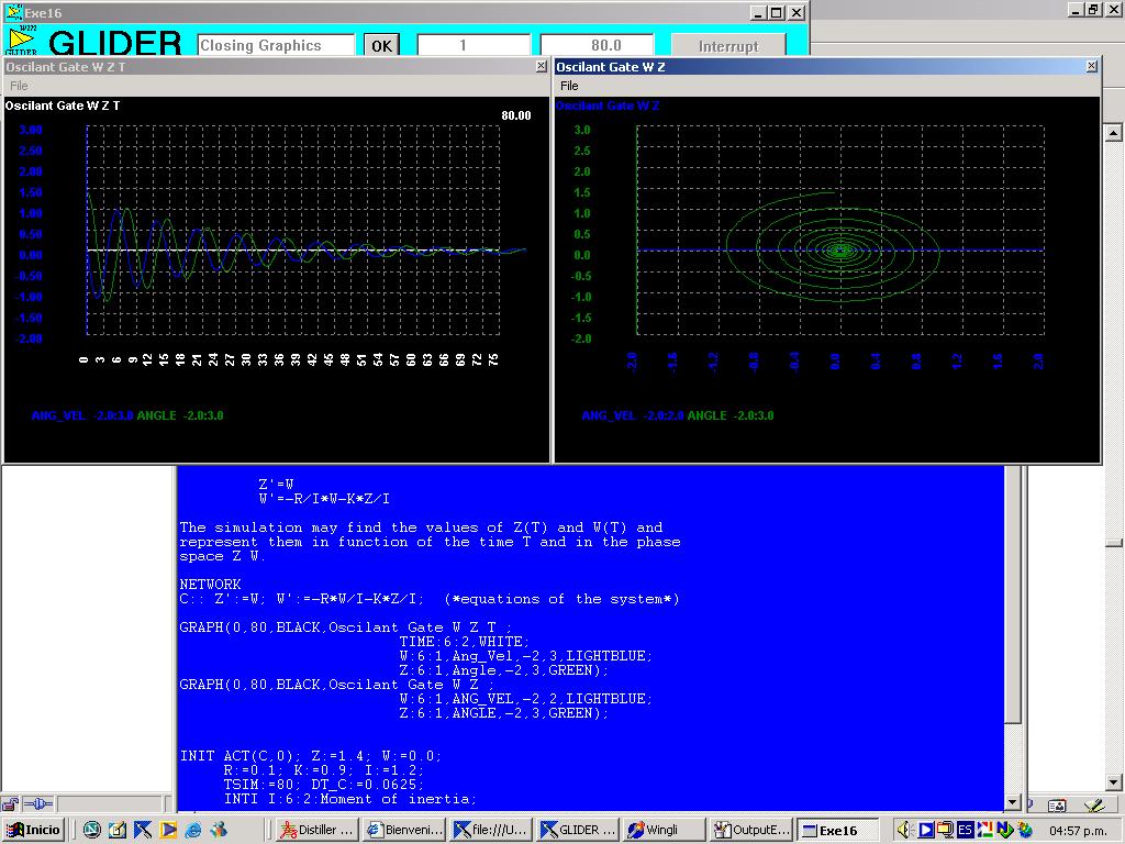
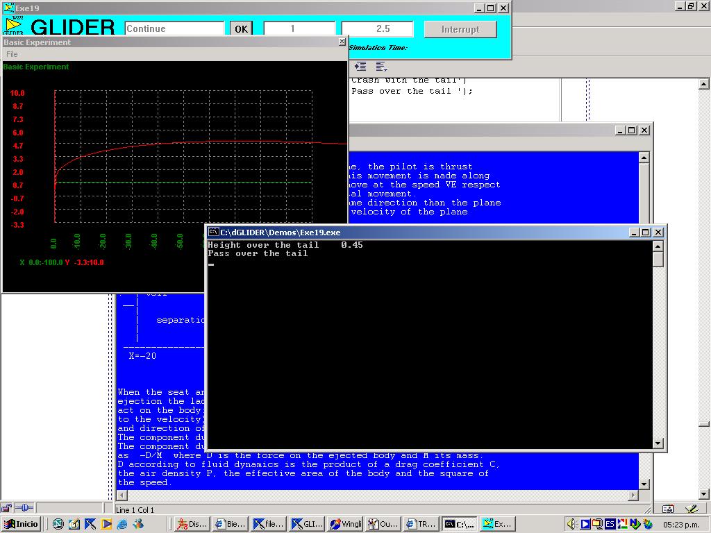
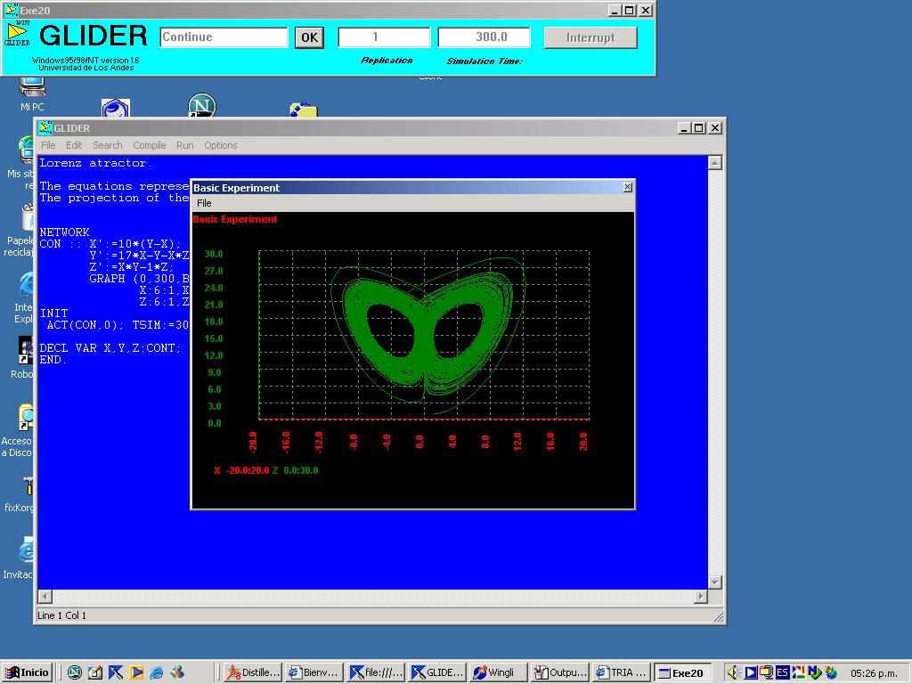